从DDPM到DDIM(三) DDPM的训练与推理

从DDPM到DDIM(三) DDPM的训练与推理

前情回顾

首先还是回顾一下之前讨论的成果。

扩散模型的结构和各个概率模型的意义。下图展示了DDPM的双向马尔可夫模型。

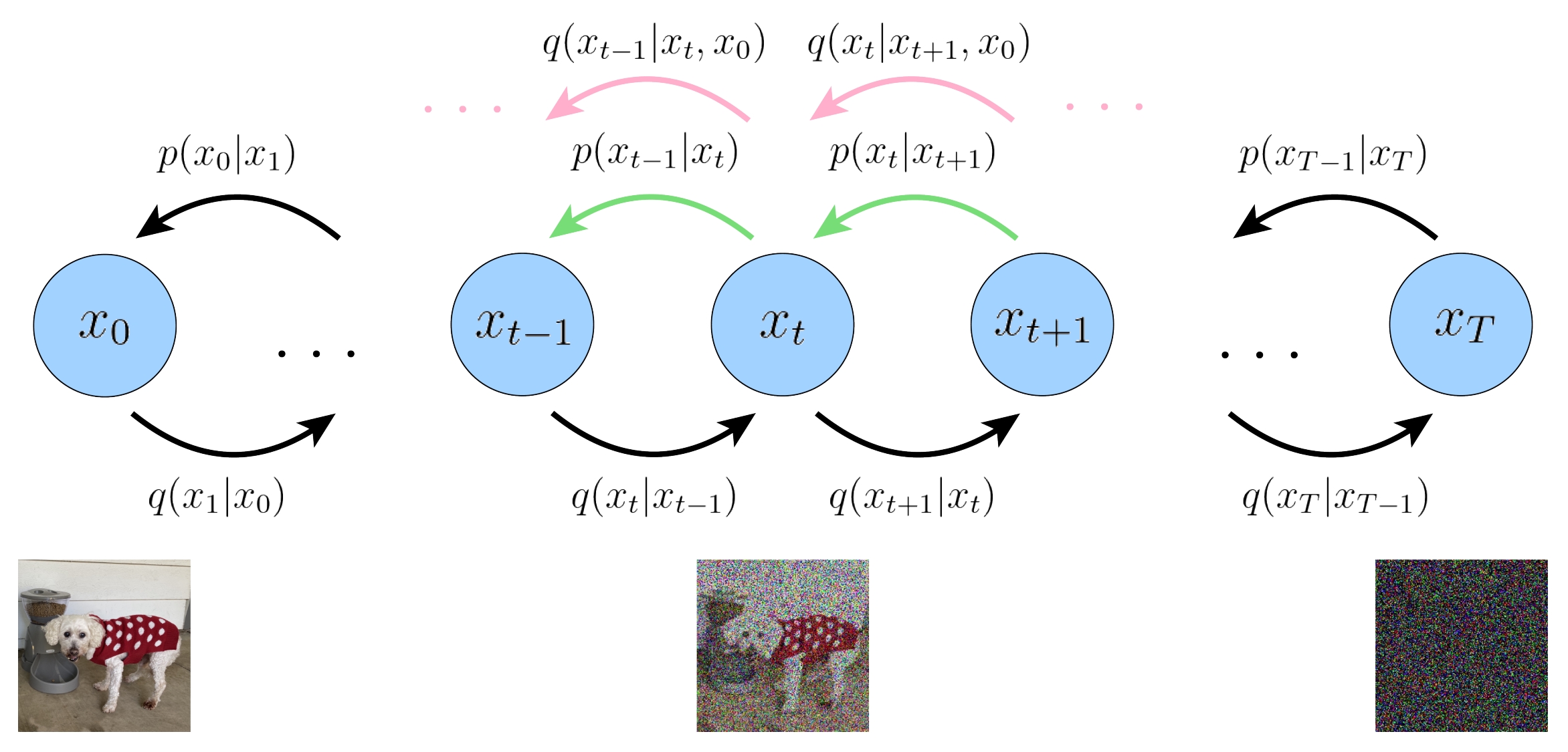
其中\(\mathbf{x}_T\)代表纯高斯噪声，\(\mathbf{x}_t, 0 < t < T\) 代表中间的隐变量, \(\mathbf{x}_0\) 代表生成的图像。

• \(q\left(\mathbf{x}_{t} | \mathbf{x}_{t-1}\right)\) 加噪过程的单步转移概率，服从高斯分布，这很好理解。
• \(q\left(\mathbf{x}_{t-1} | \mathbf{x}_{t}\right)\) 是真正的采样过程的单步转移概率，但是求解它比较困难。
• \(p_{\theta}\left(\mathbf{x}_{t-1} | \mathbf{x}_{t}\right)\) 代表的是神经网络拟合的概率，我们希望神经网络能更好地拟合采样过程的单步转移概率。
• \(q\left(\mathbf{x}_{t-1} | \mathbf{x}_{t}, \mathbf{x}_{0}\right)\)，给定最终生成结果 \(\mathbf{x}_{0}\) 的条件下，生成过程的单步转移概率。\(\mathbf{x}_{0}\) 就像有监督学习中的标签，指导着生成的方向。我们采用此概率来替代 \(q\left(\mathbf{x}_{t-1} | \mathbf{x}_{t}\right)\) 做神经网络的拟合。如果无法理解，把它当作一个无物理意义的数学上的中间变量即可。

\(p_{\theta}(\mathbf{x}_{t-1} | \mathbf{x}_{t})\) 来表示。之所以这里增加一个 \(\theta\) 下标，是因为 \(p_{\theta}(\mathbf{x}_{t-1} | \mathbf{x}_{t})\) 是用神经网络来逼近的转移概率， \(\theta\) 代表神经网络参数。

联合概率表示 扩散模型的联合概率和前向条件联合概率为：

\[\begin{aligned}
{p\left(\mathbf{x}_{0:T}\right) = p\left(\mathbf{x}_{T}\right) \prod_{t=1}^{T} p_{\theta}\left(\mathbf{x}_{t-1}|\mathbf{x}_{t}\right)}
\end{aligned} \tag{1}
\]

\[\begin{aligned}
{q\left(\mathbf{x}_{1:T} | \mathbf{x}_{0}\right) = \prod_{t=1}^T q\left(\mathbf{x}_{t} | \mathbf{x}_{t-1}\right)} \\
\end{aligned} \tag{2}
\]

概率分布的具体表达式 之前提到的各种条件概率的具体表达式为：

\[\begin{aligned}
q(\mathbf{x}_{t} | \mathbf{x}_{t-1}) &= \mathcal{N}(\mathbf{x}_t; \sqrt{\alpha_t} \mathbf{x}_{t-1}, (1 - \alpha_t) \mathbf{I}) \\
q(\mathbf{x}_{t} | \mathbf{x}_{0}) &= \mathcal{N}(\mathbf{x}_{t}; \sqrt{\overline{\alpha}_t} \mathbf{x}_{0}, (1 - \overline{\alpha}_t) \mathbf{I}) \\
q\left(\mathbf{x}_{t-1} | \mathbf{x}_{t}, \mathbf{x}_{0}\right) &= \mathcal{N}(\mathbf{x}_{t-1}; \tilde{\bm{\mu}}_{t}\left(\mathbf{x}_{t}, \mathbf{x}_{0}\right) , \tilde{\bm{\Sigma}} \left(t\right))\\
\end{aligned} \tag{3}
\]

其中

\[\begin{aligned}
\tilde{\bm{\mu}}_{t}\left(\mathbf{x}_{t}, \mathbf{x}_{0}\right) &= \frac{\left( 1 - \overline{\alpha}_{t-1} \right) \sqrt{\alpha_t}}{\left( 1 - \overline{\alpha}_{t} \right)} \mathbf{x}_{t} + \frac{\left(1 - \alpha_t\right) \sqrt{\overline{\alpha}_{t-1}}}{\left( 1 - \overline{\alpha}_{t} \right)} \mathbf{x}_{0} \\
\tilde{\bm{\Sigma}} \left(t\right) &= \frac{\left(1 - \alpha_t\right) \left( 1 - \overline{\alpha}_{t-1} \right)}{ 1 - \overline{\alpha}_{t} } \mathbf{I} = \sigma^2 \left(t\right) \mathbf{I}\\
\end{aligned}
\]

另外，\(p\left(\mathbf{x}_{T}\right)\) 服从标准高斯分布，\(p_{\theta}\left(\mathbf{x}_{t-1}|\mathbf{x}_{t}\right)\) 是我们要训练的神经网络。

根据贝叶斯公式，我们要改造的条件概率如下：

\[\begin{aligned}
q\left(\mathbf{x}_{t} | \mathbf{x}_{t-1}, \mathbf{x}_{0}\right) = \frac{\textcolor{blue}{q\left(\mathbf{x}_{t-1} | \mathbf{x}_{t}, \mathbf{x}_{0}\right)} q\left(\mathbf{x}_{t} | \mathbf{x}_{0}\right)}{q\left(\mathbf{x}_{t-1} | \mathbf{x}_{0}\right)}
\end{aligned} \tag{4}
\]

证据下界 我们原本要对生成的图像分布进行极大似然估计，但直接估计无法计算。于是我们改为最大化证据下界，然后对证据下界进行化简，现在，我们采用 \(q\left(\mathbf{x}_{t-1} | \mathbf{x}_{t}, \mathbf{x}_{0}\right)\) 重新优化证据下界：

\[\begin{aligned}
\log p\left(\mathbf{x}_0\right) &\geq \mathcal{L} \\
&= \mathbb{E}_{q\left(\mathbf{x}_{1:T} | \mathbf{x}_{0}\right)} \left[ \log \frac{p\left(\mathbf{x}_{T}\right) \prod_{t=1}^{T} p_{\theta}\left(\mathbf{x}_{t-1}|\mathbf{x}_{t}\right)}{\prod_{t=1}^T q\left(\mathbf{x}_{t} | \mathbf{x}_{t-1}\right)}\right] \\
\end{aligned} \tag{5}
\]

3.5、利用 \(q(\mathbf{x}_{t-1} | \mathbf{x}_{t}, \mathbf{x}_{0})\) 重新推导证据下界

  书接上回。我们化简证据下界的一个想法是，我们希望将 \(p_{\theta}\left(\mathbf{x}_{t-1}|\mathbf{x}_{t}\right)\) 和 \(q\left(\mathbf{x}_{t} | \mathbf{x}_{t-1}\right)\) 的每一项一一对齐；并且将含有 \(\left(\mathbf{x}_{0}, \mathbf{x}_{1}\right)\) 的项与其他项分开来。因为 \(\mathbf{x}_{0}\) 是图像，而其他随机变量是隐变量。还有一种解释是，这次我们采用了 \(q(\mathbf{x}_{t-1} | \mathbf{x}_{t}, \mathbf{x}_{0})\)，而当 \(t = 1\) 时，\(q(\mathbf{x}_{0} | \mathbf{x}_{1}, \mathbf{x}_{0})\) 看起来好像是无意义的。所以我们要将含有 \(\left(\mathbf{x}_{0}, \mathbf{x}_{1}\right)\) 的项与其他项分开。

\[\begin{aligned}
\mathcal{L} &= \mathbb{E}_{q\left(\mathbf{x}_{1:T} | \mathbf{x}_{0}\right)} \left[ \log \frac{p\left(\mathbf{x}_{T}\right) \prod_{t=1}^{T} p_{\theta}\left(\mathbf{x}_{t-1}|\mathbf{x}_{t}\right)}{\prod_{t=1}^T q\left(\mathbf{x}_{t} | \mathbf{x}_{t-1}\right)}\right] \\
&= \mathbb{E}_{q\left(\mathbf{x}_{1:T} | \mathbf{x}_{0}\right)} \left[ \log \frac{p\left(\mathbf{x}_{T}\right) p_{\theta}\left(\mathbf{x}_{0}|\mathbf{x}_{1}\right) \prod_{t=2}^{T} p_{\theta}\left(\mathbf{x}_{t-1}|\mathbf{x}_{t}\right)}{q\left(\mathbf{x}_{1} | \mathbf{x}_{0}\right) \prod_{t=2}^T q\left(\mathbf{x}_{t} | \mathbf{x}_{t-1}\right)}\right] \\
&= \mathbb{E}_{q\left(\mathbf{x}_{1:T} | \mathbf{x}_{0}\right)} \left[ \log \frac{p\left(\mathbf{x}_{T}\right) p_{\theta}\left(\mathbf{x}_{0}|\mathbf{x}_{1}\right)}{q\left(\mathbf{x}_{1} | \mathbf{x}_{0}\right)}\right] + \mathbb{E}_{q\left(\mathbf{x}_{1:T} | \mathbf{x}_{0}\right)} \left[ \log \frac{\prod_{t=2}^{T} p_{\theta}\left(\mathbf{x}_{t-1}|\mathbf{x}_{t}\right)}{\prod_{t=2}^T \textcolor{blue}{q\left(\mathbf{x}_{t} | \mathbf{x}_{t-1}, \mathbf{x}_{0}\right)}}\right]\\
&= \mathbb{E}_{q\left(\mathbf{x}_{1:T} | \mathbf{x}_{0}\right)} \left[ \log \frac{p\left(\mathbf{x}_{T}\right) p_{\theta}\left(\mathbf{x}_{0}|\mathbf{x}_{1}\right)}{q\left(\mathbf{x}_{1} | \mathbf{x}_{0}\right)}\right] + \mathbb{E}_{q\left(\mathbf{x}_{1:T} | \mathbf{x}_{0}\right)} \left[ \log \frac{\prod_{t=2}^{T} p_{\theta}\left(\mathbf{x}_{t-1}|\mathbf{x}_{t}\right)}{\prod_{t=2}^T \textcolor{blue}{\frac{q\left(\mathbf{x}_{t-1} | \mathbf{x}_{t}, \mathbf{x}_{0}\right) q\left(\mathbf{x}_{t} | \mathbf{x}_{0}\right)}{q\left(\mathbf{x}_{t-1} | \mathbf{x}_{0}\right)}}}\right]\\
&= \mathbb{E}_{q\left(\mathbf{x}_{1:T} | \mathbf{x}_{0}\right)} \left[ \log \frac{p\left(\mathbf{x}_{T}\right) p_{\theta}\left(\mathbf{x}_{0}|\mathbf{x}_{1}\right)}{q\left(\mathbf{x}_{1} | \mathbf{x}_{0}\right)}\right] + \mathbb{E}_{q\left(\mathbf{x}_{1:T} | \mathbf{x}_{0}\right)} \left[ \log \prod_{t=2}^{T} \frac{q\left(\mathbf{x}_{t-1} | \mathbf{x}_{0}\right)}{q\left(\mathbf{x}_{t} | \mathbf{x}_{0}\right)}\right] + \mathbb{E}_{q\left(\mathbf{x}_{1:T} | \mathbf{x}_{0}\right)} \left[ \log \frac{\prod_{t=2}^{T} p_{\theta}\left(\mathbf{x}_{t-1}|\mathbf{x}_{t}\right)}{\prod_{t=2}^T \textcolor{blue}{q\left(\mathbf{x}_{t-1} | \mathbf{x}_{t}, \mathbf{x}_{0}\right)}}\right]\\
&= \mathbb{E}_{q\left(\mathbf{x}_{1:T} | \mathbf{x}_{0}\right)} \left[ \log \frac{p\left(\mathbf{x}_{T}\right) p_{\theta}\left(\mathbf{x}_{0}|\mathbf{x}_{1}\right)}{\textcolor{red}{q\left(\mathbf{x}_{1} | \mathbf{x}_{0}\right)}}\right] + \mathbb{E}_{q\left(\mathbf{x}_{1:T} | \mathbf{x}_{0}\right)} \left[ \log \frac{\textcolor{red}{q\left(\mathbf{x}_{1} | \mathbf{x}_{0}\right)}}{q\left(\mathbf{x}_{T} | \mathbf{x}_{0}\right)}\right] + \mathbb{E}_{q\left(\mathbf{x}_{1:T} | \mathbf{x}_{0}\right)} \left[ \log \frac{\prod_{t=2}^{T} p_{\theta}\left(\mathbf{x}_{t-1}|\mathbf{x}_{t}\right)}{\prod_{t=2}^T q\left(\mathbf{x}_{t-1} | \mathbf{x}_{t}, \mathbf{x}_{0}\right)}\right]\\
&= \mathbb{E}_{q\left(\mathbf{x}_{1:T} | \mathbf{x}_{0}\right)} \left[ \log \frac{p\left(\mathbf{x}_{T}\right) p_{\theta}\left(\mathbf{x}_{0}|\mathbf{x}_{1}\right)}{q\left(\mathbf{x}_{T} | \mathbf{x}_{0}\right)}\right] + \sum_{t=2}^{T} \mathbb{E}_{q\left(\mathbf{x}_{1:T} | \mathbf{x}_{0}\right)} \left[ \log \frac{p_{\theta}\left(\mathbf{x}_{t-1}|\mathbf{x}_{t}\right)}{q\left(\mathbf{x}_{t-1} | \mathbf{x}_{t}, \mathbf{x}_{0}\right)}\right] \quad\quad 红色消去，乘法变加法\\
&= \textcolor{Skyblue}{\mathbb{E}_{q\left(\mathbf{x}_{1:T} | \mathbf{x}_{0}\right)} \left[ \log p_{\theta}\left(\mathbf{x}_{0}|\mathbf{x}_{1}\right)\right]} + \textcolor{Darkred}{\mathbb{E}_{q\left(\mathbf{x}_{1:T} | \mathbf{x}_{0}\right)} \left[ \log \frac{p\left(\mathbf{x}_{T}\right)}{q\left(\mathbf{x}_{T} | \mathbf{x}_{0}\right)}\right]} + \textcolor{Darkgreen}{\sum_{t=2}^{T} \mathbb{E}_{q\left(\mathbf{x}_{1:T} | \mathbf{x}_{0}\right)} \left[ \log \frac{p_{\theta}\left(\mathbf{x}_{t-1}|\mathbf{x}_{t}\right)}{q\left(\mathbf{x}_{t-1} | \mathbf{x}_{t}, \mathbf{x}_{0}\right)}\right]} \\
\end{aligned}
\]

与之前一样，上式三项也分别代表三部分：重建项、先验匹配项 和 一致项。

• 重建项。顾名思义，这是对最后构图的预测概率。给定预测的最后一个隐变量 \(\mathbf{x}_{1}\)，预测生成的图像 \(\mathbf{x}_{0}\) 的对数概率。
• 先验匹配项。 这一项描述的是扩散过程的最后一步生成的高斯噪声与纯高斯噪声的相似度，与之前相比，这一项的 \(q\) 部分的条件改为了 \(\mathbf{x}_{0}\)。同样，这一项并没有神经网络参数，所以不需要优化，后续网络训练的时候可以将这一项舍去。
• 一致项。这一项与之前有两点不同。其一，与之前相比，不再有错位比较。其二，这匹配目标改为了由 \(p_{\theta}\left(\mathbf{x}_{t}|\mathbf{x}_{t+1}\right)\) 向 \(q\left(\mathbf{x}_{t-1} | \mathbf{x}_{t}, \mathbf{x}_{0}\right)\) 匹配，而之前是和扩散过程的单步转移概率 \(q\left(\mathbf{x}_{t}|\mathbf{x}_{t-1}\right)\) 匹配。更加合理。

类似地，与之前的操作一样，我们将上式的数学期望下角标中的无关的随机变量约去(积分为1)，然后转化成KL散度的形式。我们看 先验匹配项 和 一致项。

\[\begin{aligned}
\textcolor{Darkred}{\mathbb{E}_{q\left(\mathbf{x}_{1:T} | \mathbf{x}_{0}\right)} \left[ \log \frac{p\left(\mathbf{x}_{T}\right)}{q\left(\mathbf{x}_{T} | \mathbf{x}_{0}\right)}\right]} &= \int q\left(\mathbf{x}_{1:T} | \mathbf{x}_{0}\right) \log \frac{p\left(\mathbf{x}_{T}\right)}{q\left(\mathbf{x}_{T} | \mathbf{x}_{0}\right)} d \mathbf{x}_{1:T}\\
&= \int q\left(\mathbf{x}_{T} | \mathbf{x}_{0}\right) \log \frac{p\left(\mathbf{x}_{T}\right)}{q\left(\mathbf{x}_{T} | \mathbf{x}_{0}\right)} d \mathbf{x}_{T}\\
&= -\mathbb{D}_{\text{KL}} \left(q\left(\mathbf{x}_{T} | \mathbf{x}_{0}\right) \| p\left(\mathbf{x}_{T}\right)\right)
\end{aligned}
\]

\[\begin{aligned}
\textcolor{Darkgreen}{\mathbb{E}_{q\left(\mathbf{x}_{1:T} | \mathbf{x}_{0}\right)} \left[ \log \frac{p_{\theta}\left(\mathbf{x}_{t-1}|\mathbf{x}_{t}\right)}{q\left(\mathbf{x}_{t-1} | \mathbf{x}_{t}, \mathbf{x}_{0}\right)}\right]} &= \int q\left(\mathbf{x}_{1:T} | \mathbf{x}_{0}\right) \log \frac{p_{\theta}\left(\mathbf{x}_{t-1}|\mathbf{x}_{t}\right)}{q\left(\mathbf{x}_{t-1} | \mathbf{x}_{t}, \mathbf{x}_{0}\right)} d \mathbf{x}_{1:T}\\
&= \int q\left(\mathbf{x}_{t}, \mathbf{x}_{t-1} | \mathbf{x}_{0}\right) \log \frac{p_{\theta}\left(\mathbf{x}_{t-1}|\mathbf{x}_{t}\right)}{q\left(\mathbf{x}_{t-1} | \mathbf{x}_{t}, \mathbf{x}_{0}\right)} d \mathbf{x}_{t} d\mathbf{x}_{t-1}\\
&= \int q\left(\mathbf{x}_{t} | \mathbf{x}_{0}\right) q\left(\mathbf{x}_{t-1} | \mathbf{x}_{t}, \mathbf{x}_{0}\right) \log \frac{p_{\theta}\left(\mathbf{x}_{t-1}|\mathbf{x}_{t}\right)}{q\left(\mathbf{x}_{t-1} | \mathbf{x}_{t}, \mathbf{x}_{0}\right)} d \mathbf{x}_{t} d\mathbf{x}_{t-1}\\
&= \int q\left(\mathbf{x}_{t} | \mathbf{x}_{0}\right) \mathbb{D}_{\text{KL}} \left(q\left(\mathbf{x}_{t-1} | \mathbf{x}_{t}, \mathbf{x}_{0}\right) \| p_{\theta}\left(\mathbf{x}_{t-1}|\mathbf{x}_{t}\right)\right) d \mathbf{x}_{t} \\
&= -\mathbb{E}_{q\left(\mathbf{x}_{t} | \mathbf{x}_{0}\right)} \left[ \mathbb{D}_{\text{KL}} \left(q\left(\mathbf{x}_{t-1} | \mathbf{x}_{t}, \mathbf{x}_{0}\right) \| p_{\theta}\left(\mathbf{x}_{t-1}|\mathbf{x}_{t}\right)\right)\right]
\end{aligned}
\]

重建项也类似，期望下角标的概率中，除了随机变量 \(\mathbf{x}_1\) 之外都可以约掉。最后，我们终于得出证据下界的KL散度形式：

\[\begin{aligned}
\mathcal{L} &= \textcolor{Skyblue}{\mathbb{E}_{q\left(\mathbf{x}_{1} | \mathbf{x}_{0}\right)} \left[ \log p_{\theta}\left(\mathbf{x}_{0}|\mathbf{x}_{1}\right)\right]} - \textcolor{Darkred}{\mathbb{D}_{\text{KL}} \left(q\left(\mathbf{x}_{T} | \mathbf{x}_{0}\right) \| p\left(\mathbf{x}_{T}\right)\right)} \\
&- \textcolor{Darkgreen}{\sum_{t=2}^{T} \mathbb{E}_{q\left(\mathbf{x}_{t} | \mathbf{x}_{0}\right)} \left[ \mathbb{D}_{\text{KL}} \left(q\left(\mathbf{x}_{t-1} | \mathbf{x}_{t}, \mathbf{x}_{0}\right) \| p_{\theta}\left(\mathbf{x}_{t-1}|\mathbf{x}_{t}\right)\right)\right]} \\
\end{aligned} \tag{6}
\]

  下面聊聊数学期望的下角标的物理意义是。以重建项为例，下角标为 \(q\left(\mathbf{x}_{1} | \mathbf{x}_{0}\right)\)，代表用 \(\mathbf{x}_{0}\) 加噪一步生成 \(\mathbf{x}_{1}\)，然后用 \(\mathbf{x}_{1}\) 输入到神经网络中得到估计的 \(\mathbf{x}_{0}\) 的分布，然后最大化这个对数似然概率。而数学期望代表了多个图片，一个 epoch 之后取平均作为期望。一致项也类似，只是用 \(\mathbf{x}_{0}\) 生成 \(\mathbf{x}_{t}\)，然后通过神经网络计算与 \(q\left(\mathbf{x}_{t-1} | \mathbf{x}_{t}, \mathbf{x}_{0}\right)\) 的KL散度。这实际上就是蒙特卡洛估计。

所以，我们需要计算loss的项有两个，一个是重建项中的对数部分，一个是一致项中的KL散度。至于数学期望和下角标，我们并不需要展开计算，而是在训练的时候用多个图片并分别添加不同程度的噪声来替代。

4、训练过程

  下面我们利用 (3) 式对证据下界 (6) 式做进一步展开。从DDPM到DDIM(二) 这篇文章讲过，在 \(\beta_t\) 很小的前提下，\(p_{\theta}\left(\mathbf{x}_{t-1}|\mathbf{x}_{t}\right)\) 也服从高斯分布。因为 \(p_{\theta}\left(\mathbf{x}_{t-1}|\mathbf{x}_{t}\right)\) 的训练目标是匹配 \(q\left(\mathbf{x}_{t-1} | \mathbf{x}_{t}, \mathbf{x}_{0}\right)\)，我们也写成高斯分布的形式，并与 \(q\left(\mathbf{x}_{t-1} | \mathbf{x}_{t}, \mathbf{x}_{0}\right)\) 的形式做对比。

\[\begin{aligned}
q\left(\mathbf{x}_{t-1} | \mathbf{x}_{t}, \mathbf{x}_{0}\right) &= \mathcal{N}(\mathbf{x}_{t-1}; \tilde{\bm{\mu}}_{t}\left(\mathbf{x}_{t}, \mathbf{x}_{0}\right) , \tilde{\bm{\Sigma}} \left(t\right))\\
&= \frac{1}{\sqrt{2 \pi} \sigma \left(t\right)} \exp \left[ -\frac{1}{2} \left(\mathbf{x}_{t-1} - \tilde{\bm{\mu}}_{t}\left(\mathbf{x}_{t}, \mathbf{x}_{0}\right)\right)^T \tilde{\bm{\Sigma}}^{-1} \left(t\right) \left(\mathbf{x}_{t-1} - \tilde{\bm{\mu}}_{t}\left(\mathbf{x}_{t}, \mathbf{x}_{0}\right)\right)\right]\\
p_{\theta}\left(\mathbf{x}_{t-1}|\mathbf{x}_{t}\right) &= \mathcal{N}(\mathbf{x}_{t-1}; \textcolor{blue}{\tilde{\bm{\mu}}_{\theta}\left(\mathbf{x}_{t}, t\right)} , \tilde{\bm{\Sigma}} \left(t\right))\\
&= \frac{1}{\sqrt{2 \pi} \sigma \left(t\right)} \exp \left[ -\frac{1}{2} \left(\mathbf{x}_{t-1} - \tilde{\bm{\mu}}_{\theta}\left(\mathbf{x}_{t}, t\right)\right)^T \tilde{\bm{\Sigma}}^{-1} \left(t\right) \left(\mathbf{x}_{t-1} - \tilde{\bm{\mu}}_{\theta}\left(\mathbf{x}_{t}, t\right)\right)\right]\\
\end{aligned}
\]

这里 \(p_{\theta}\left(\mathbf{x}_{t-1}|\mathbf{x}_{t}\right)\) 的均值 \(\textcolor{blue}{\tilde{\bm{\mu}}_{\theta}\left(\mathbf{x}_{t}, t\right)}\) 是神经网络输出，方差我们采用和 \(q\left(\mathbf{x}_{t-1} | \mathbf{x}_{t}, \mathbf{x}_{0}\right)\) 一样的方差。神经网络 \(\textcolor{blue}{\tilde{\bm{\mu}}_{\theta}\left(\mathbf{x}_{t}, t\right)}\) 的输入有两个，第一个是 \(\mathbf{x}_{t}\)，这是显然的，还有一个输入时时刻 \(t\)，因为当然，方差也可以作为神经网络来训练，但是DDPM原文中做过实验，这样效果并不显著。因此，上述两个均值两个方差中，只有蓝色的 \(\textcolor{blue}{\tilde{\bm{\mu}}_{\theta}\left(\mathbf{x}_{t}, t\right)}\) 是未知的，另外三个量都是已知量。

根据 (6) 式，我们只需要计算 重建项 和 一致项，先验匹配项没有训练参数。下面分别计算：

\[\begin{aligned}
\textcolor{Skyblue}{ \log p_{\theta}\left(\mathbf{x}_{0}|\mathbf{x}_{1}\right) } &= -\frac{1}{2 \sigma^2 \left(t\right)} \Vert \mathbf{x}_{0} - \tilde{\bm{\mu}}_{\theta}\left(\mathbf{x}_{1}, 1\right) \Vert_2^2 + \text{const}\\
\end{aligned}
\]

其中 \(\text{const}\) 代表某个常数。

  下面计算一致项，即KL散度。高斯分布的KL散度是有公式的，我们不加证明地给出，若需要证明，可以查阅维基百科。两个 \(d\) 维随机变量服从高斯分布 \(Q = \mathcal{N}(\bm{\mu}_1, \bm{\Sigma}_1)\) , $P = \mathcal{N}(\bm{\mu}_2, \bm{\Sigma}_2) $，其中 \(\bm{\mu}_1, \bm{\mu}_2 \in \mathbb{R}^{d}, \bm{\Sigma}_1, \bm{\Sigma}_2 \in \mathbb{R}^{d \times d}\) 二者的Kullback-Leibler 散度（KL散度）可以用以下公式计算：

\[\begin{aligned}
\mathbb{D}_{\text{KL}}(Q \| P) = \frac{1}{2} \left[\log \frac{\det \bm{\Sigma}_2}{\det \bm{\Sigma}_1} - d + \text{tr}(\bm{\Sigma}_2^{-1} \bm{\Sigma}_1) + (\bm{\mu}_2 - \bm{\mu}_1)^T \bm{\Sigma}_2^{-1} (\bm{\mu}_2 - \bm{\mu}_1)\right]\\
\end{aligned}
\]

下面我们将一致项代入上述公式：

\[\begin{aligned}
\textcolor{Darkgreen}{\mathbb{D}_{\text{KL}} \left(q\left(\mathbf{x}_{t-1} | \mathbf{x}_{t}, \mathbf{x}_{0}\right) \| p_{\theta}\left(\mathbf{x}_{t-1}|\mathbf{x}_{t}\right)\right)} &= \frac{1}{2} \left[\log 1 - d + d + \Vert\tilde{\bm{\mu}}_{\theta}\left(\mathbf{x}_{t}, t\right) - \tilde{\bm{\mu}}_{t}\left(\mathbf{x}_{t}, \mathbf{x}_{0}\right)\Vert_2^2 / \sigma^2 \left(t\right)\right]\\
&= \frac{1}{2 \sigma^2 \left(t\right)} \Vert\tilde{\bm{\mu}}_{\theta}\left(\mathbf{x}_{t}, t\right) - \tilde{\bm{\mu}}_{t}\left(\mathbf{x}_{t}, \mathbf{x}_{0}\right)\Vert_2^2\\
\end{aligned} \tag{7}
\]

从上两个式子可以看出，\(\tilde{\bm{\mu}}_{\theta}\left(\mathbf{x}_{t}, t\right)\) 在 \(t > 0\) 的时候，目标是匹配 \(\tilde{\bm{\mu}}_{t}\left(\mathbf{x}_{t}, \mathbf{x}_{0}\right)\)。我们的研究哲学是，只要有解析形式，我们就将解析形式展开，直到某个变量没有解析解，这时候才会用神经网络拟合，这样可以最大化地保证拟合的效果。比如我们为了拟合一个二次函数 \(f(x) = a x^2 + 3 x + 2\)，其中 \(a\) 是未知量，我们应该设计一个神经网络来估计 \(a\)，而不应该用神经网络来估计 \(f(x)\)，因为前者确保了神经网络估计出来的函数是二次函数，而后者则有更多的不确定性。

  为了更好地匹配，我们展开 \(\tilde{\bm{\mu}}_{t}\left(\mathbf{x}_{t}, \mathbf{x}_{0}\right)\) 中的解析形式。

\[\begin{aligned}
\tilde{\bm{\mu}}_{t}\left(\mathbf{x}_{t}, \mathbf{x}_{0}\right) &= \frac{\left( 1 - \overline{\alpha}_{t-1} \right) \sqrt{\alpha_t}}{\left( 1 - \overline{\alpha}_{t} \right)} \mathbf{x}_{t} + \frac{\left(1 - \alpha_t\right) \sqrt{\overline{\alpha}_{t-1}}}{\left( 1 - \overline{\alpha}_{t} \right)} \mathbf{x}_{0} \\
\tilde{\bm{\mu}}_{\theta}\left(\mathbf{x}_{t}, t\right) &= \frac{\left( 1 - \overline{\alpha}_{t-1} \right) \sqrt{\alpha_t}}{\left( 1 - \overline{\alpha}_{t} \right)} \mathbf{x}_{t} + \frac{\left(1 - \alpha_t\right) \sqrt{\overline{\alpha}_{t-1}}}{\left( 1 - \overline{\alpha}_{t} \right)} \tilde{\mathbf{x}}_{\theta} \left(\mathbf{x}_{t}, t\right) \\
\end{aligned} \tag{8}
\]

\(\tilde{\bm{\mu}}_{\theta}\left(\mathbf{x}_{t}, t\right)\) 展开的形式与 \(\tilde{\bm{\mu}}_{t}\left(\mathbf{x}_{t}, \mathbf{x}_{0}\right)\) 相同。第一项是与 \(\mathbf{x}_{t}\) 相关的，因为 \(\mathbf{x}_{t}\) 是输入，所以保持不变，但是 \(\mathbf{x}_{0}\) 是未知量，所以我们还是用神经网络来替代，神经网络的输入同样也是 \(\mathbf{x}_{t}\) 和 \(t\)。将 (8) 式代入 (7) 式，有：

\[\begin{aligned}
\textcolor{Darkgreen}{\mathbb{D}_{\text{KL}} \left(q\left(\mathbf{x}_{t-1} | \mathbf{x}_{t}, \mathbf{x}_{0}\right) \| p_{\theta}\left(\mathbf{x}_{t-1}|\mathbf{x}_{t}\right)\right)} &= \frac{1}{2 \sigma^2 \left(t\right)} \Vert\tilde{\bm{\mu}}_{\theta}\left(\mathbf{x}_{t}\right) - \tilde{\bm{\mu}}_{t}\left(\mathbf{x}_{t}, \mathbf{x}_{0}\right)\Vert_2^2 \\
&= \frac{1}{2 \sigma^2 \left(t\right)} \frac{\left(1 - \alpha_t\right)^2 \overline{\alpha}_{t-1}}{\left( 1 - \overline{\alpha}_{t} \right)^2} \Vert\mathbf{x}_{0} - \tilde{\mathbf{x}}_{\theta} \left(\mathbf{x}_{t}, t\right)\Vert_2^2 \\
\end{aligned}
\]

重建项也可以继续化简，注意到 \(\beta_0 = 0, \alpha_0 = 1, \overline{\alpha}_{0} = 1, \overline{\alpha}_{1} = \alpha_1\)：

\[\begin{aligned}
\textcolor{Skyblue}{ \log p_{\theta}\left(\mathbf{x}_{0}|\mathbf{x}_{1}\right) } &= -\frac{1}{2 \sigma^2 \left(t\right)} \Vert \mathbf{x}_{0} - \tilde{\bm{\mu}}_{\theta}\left(\mathbf{x}_{1}, 1\right) \Vert_2^2 + \text{const}\\
&= -\frac{1}{2 \sigma^2 \left(t\right)} \Vert \mathbf{x}_{0} - \frac{\left( 1 - \overline{\alpha}_{0} \right) \sqrt{\alpha_1}}{\left( 1 - \overline{\alpha}_{1} \right)} \mathbf{x}_{t} + \frac{\left(1 - \alpha_1\right) \sqrt{\overline{\alpha}_{0}}}{\left( 1 - \overline{\alpha}_{1} \right)} \tilde{\mathbf{x}}_{\theta} \left(\mathbf{x}_{1}, t\right) \Vert_2^2 + \text{const}\\
&= -\frac{1}{2 \sigma^2 \left(t\right)} \Vert \mathbf{x}_{0} - \tilde{\mathbf{x}}_{\theta} \left(\mathbf{x}_{1}, t\right) \Vert_2^2 + \text{const}\\
&= -\frac{1}{2 \sigma^2 \left(t\right)} \frac{\left(1 - \alpha_1\right)^2 \overline{\alpha}_{0}}{\left( 1 - \overline{\alpha}_{1} \right)^2} \Vert\mathbf{x}_{0} - \tilde{\mathbf{x}}_{\theta} \left(\mathbf{x}_{t}, t\right)\Vert_2^2 + \text{const} \\
\end{aligned}
\]

上式最后一行是为了与KL散度的形式保持一致。经过这么长时间的努力，我们终于将证据下界化为最简形式。我们把我们计算出的重建项和一致项代入到 (6) 式，并舍弃和神经网络参数无关的先验匹配项，有：

\[\begin{aligned}
\mathcal{L} &= - \sum_{t=1}^{T} \mathbb{E}_{q\left(\mathbf{x}_{t} | \mathbf{x}_{0}\right)} \left[ \frac{1}{2 \sigma^2 \left(t\right)} \frac{\left(1 - \alpha_t\right)^2 \overline{\alpha}_{t-1}}{\left( 1 - \overline{\alpha}_{t} \right)^2} \Vert\mathbf{x}_{0} - \tilde{\mathbf{x}}_{\theta} \left(\mathbf{x}_{t}, t\right)\Vert_2^2 \right] \\
\end{aligned} \tag{9}
\]

因为前面有个负号，所以最大化证据下界等价于最小化以下损失函数：

\[\textcolor{blue}{\boldsymbol{\theta}^*=\underset{\boldsymbol{\theta}}{\operatorname{argmin}} \sum_{t=1}^T \frac{1}{2 \sigma^2(t)} \frac{\left(1-\alpha_t\right)^2 \overline{\alpha}_{t-1}}{\left(1-\overline{\alpha}_t\right)^2} \mathbb{E}_{q\left(\mathbf{x}_t \mid \mathbf{x}_0\right)}\left[\Vert\tilde{\mathbf{x}}_{\boldsymbol{\theta}}\left(\mathbf{x}_t, t\right)-\mathbf{x}_0\Vert_2^2\right]}
\]

理解上式也很简单。首先我们看每一项的权重 \(\frac{1}{2 \sigma^2(t)} \frac{\left(1-\alpha_t\right)^2 \overline{\alpha}_{t-1}}{\left(1-\overline{\alpha}_t\right)^2}\)，这表示了马尔可夫链每一个阶段预测损失的权重，DDPM论文的实验证明，忽略此权重影响不大，所以我们继续简化为：

\[\textcolor{blue}{\boldsymbol{\theta}^*=\underset{\boldsymbol{\theta}}{\operatorname{argmin}} \sum_{t=1}^T \mathbb{E}_{q\left(\mathbf{x}_t \mid \mathbf{x}_0\right)}\left[\Vert\tilde{\mathbf{x}}_{\boldsymbol{\theta}}\left(\mathbf{x}_t, t\right)-\mathbf{x}_0\Vert_2^2\right]}
\]

  其实现方式就是给你一张图像 \(\mathbf{x}_0\)，然后分别按照不同的步骤加噪，最多加到 \(T\) 步噪声，得到 \(\mathbf{x}_1, \mathbf{x}_2, ..., \mathbf{x}_T\) 个隐变量。如下图所示，由于多步转移概率的性质，我们可以从 \(\mathbf{x}_0\) 一步加噪到任意一个噪声阶段。

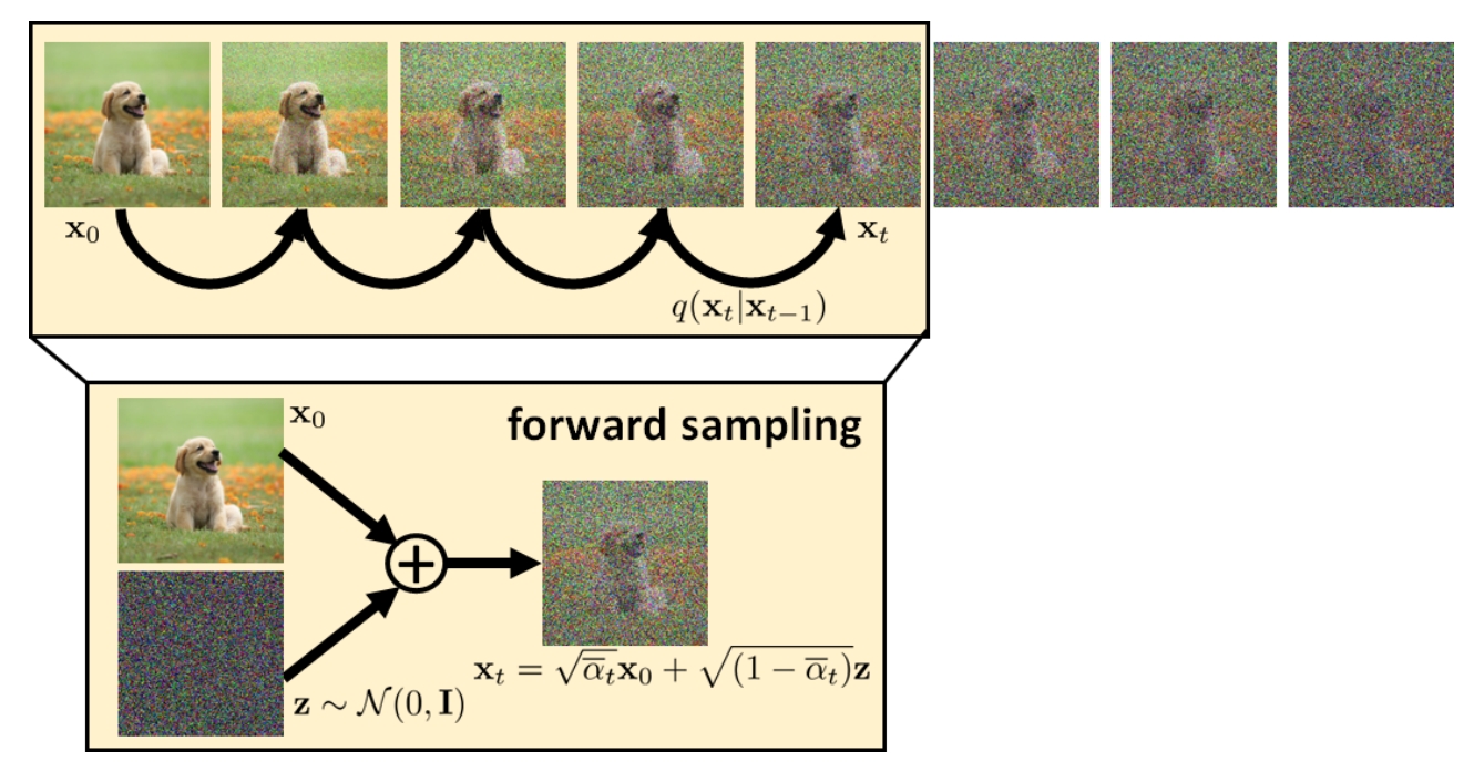
  然后将这些隐变量分别送入神经网络，输出与 \(\mathbf{x}_0\) 计算二范数Loss，然后所有的Loss取平均。然而，实际实现的时候，我们不仅仅只有一张图，而是有很多张图。送入神经网络的时候也是以一个 batch 的形式处理的，如果每张图片都加这么多次噪声，那训练的工作量就会非常巨大。所以实际上我们采用这样的方式：假设一个batch中有 \(N\) 张图片，对于这 \(N\) 张图片分别添加不同阶段的高斯噪声，图像添加噪声的程度也是随机的，比如第一张图像加噪 \(10\) 步，第二张图像加噪 \(910\) 步，等等。然后分别输入加噪后的隐变量和时刻信息，神经网络的输出与每一张原始图像分别做二范数loss，最后平均。这样相比于只给一张图像加 \(1000\) 种不同的噪声的优势是防止在一张图像上过拟合，然后陷入局部极小。下面我们给出具体的训练算法流程：

---

Algorithm 1 . Training a Deniosing Diffusion Probabilistic Model. (Version: Predict image)

For every image \(\mathbf{x}_0\) in your training dataset:

• Repeat the following steps until convergence.
• Pick a random time stamp \(t \sim \text{Uniform}[1, T]\).
• Draw a sample \(\mathbf{x}_{t} \sim q\left(\mathbf{x}_{t} | \mathbf{x}_{t}\right)\), i.e.

\[\mathbf{x}_{t} = \sqrt{\overline{\alpha}_t} \mathbf{x}_{0} + \sqrt{1 - \overline{\alpha}_t} \epsilon, \quad \epsilon \sim \mathcal{N}(\mathbf{0}, \mathbf{I})
\]

• Take gradient descent step on

\[\nabla_{\boldsymbol{\theta}} \Vert \tilde{\mathbf{x}}_{\boldsymbol{\theta}}\left(\mathbf{x}_t, t\right)-\mathbf{x}_0 \Vert_2^2
\]

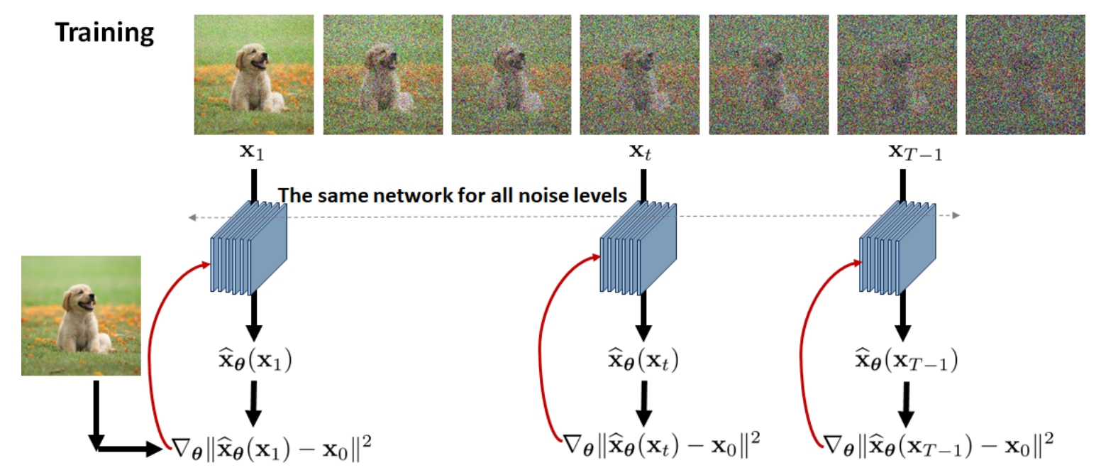
You can do this in batches, just like how you train any other neural networks. Note that, here, you are training one denoising network \(\tilde{\mathbf{x}}_{\boldsymbol{\theta}}\) for all noisy conditions.

---

采用batch来训练的话，就对每个图片分别同时进行上述操作，值得注意的是，神经网络参数只有一个，无论是哪一个 \(t\) 步去噪，其不同只有输入的不同，而神经网络只有 \(\tilde{\mathbf{x}}_{\boldsymbol{\theta}}\) 一个。训练示意图如下：

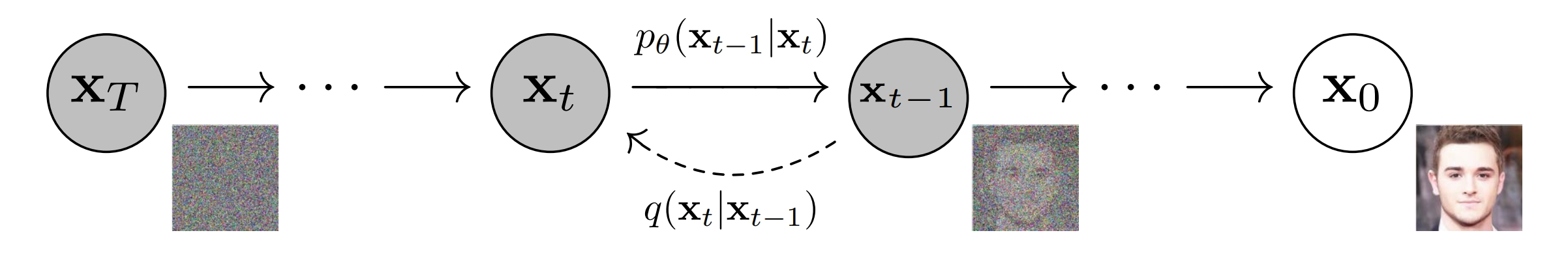
  说句题外话，其实DDPM的原文很具有误导性，如下图的DDPM的原图。从这张图上看，或许有些同学以为神经网络是输入 \(\mathbf{x}_{t}\) 来预测 \(\mathbf{x}_{t-1}\)，实际上并非如此。是输入 \(\mathbf{x}_{t}\) 来预测 \(\mathbf{x}_{0}\)，原因就是我们采用 \(q\left(\mathbf{x}_{t-1} | \mathbf{x}_{t}, \mathbf{x}_{0}\right)\) 来作为拟合目标，目标是匹配其均值 \(\tilde{\bm{\mu}}_{t}\left(\mathbf{x}_{t}, \mathbf{x}_{0}\right)\)，而不是匹配 \(\mathbf{x}_{t-1}\)。而 \(\tilde{\bm{\mu}}_{t}\left(\mathbf{x}_{t}, \mathbf{x}_{0}\right)\) 恰好是 \(\mathbf{x}_{0}\) 的函数，所以我们在训练上的时候实际上是输入 \(\mathbf{x}_{t}\) 用神经网络来预测 \(\mathbf{x}_{0}\)。而采样过程才是一步一步采样的。正因为训练时候神经网络拟合的对象并不是 \(\mathbf{x}_{t-1}\)，所以就给了我们在采样过程中的加速的空间，这就是后话了。

5、推理过程

  大家先别翻论文，你觉得最简单的一个生成图像的想法是什么。我当时就想过，既然神经网络 \(\tilde{\mathbf{x}}_{\boldsymbol{\theta}}\) 是输入 \(\mathbf{x}_{t}\) 来预测 \(\mathbf{x}_{0}\)，那么我们直接给他一个随机噪声，一步生成图像不行吗？这个问题存疑，因为最新的研究确实有单步图像生成的，不过笔者还没有精读，就暂不评价。

  按照马尔可夫性质，还是用 \(p_{\theta}\left(\mathbf{x}_{t-1} | \mathbf{x}_{t}\right)\) 一步一步做蒙特卡洛生成：

\[\begin{aligned}
\mathbf{x}_{t-1} &\sim p_{\theta}\left(\mathbf{x}_{t-1} | \mathbf{x}_{t}\right) = \mathcal{N}(\mathbf{x}_{t-1}; \tilde{\bm{\mu}}_{\theta}\left(\mathbf{x}_{t}, t\right) , \sigma^2 \left(t\right) \mathbf{I}) \\
\mathbf{x}_{t-1} &= \tilde{\bm{\mu}}_{\theta}\left(\mathbf{x}_{t}, t\right) + \sigma^2 \left(t\right) \bm{\epsilon} \\
&= \frac{\left( 1 - \overline{\alpha}_{t-1} \right) \sqrt{\alpha_t}}{\left( 1 - \overline{\alpha}_{t} \right)} \mathbf{x}_{t} + \frac{\left(1 - \alpha_t\right) \sqrt{\overline{\alpha}_{t-1}}}{\left( 1 - \overline{\alpha}_{t} \right)} \tilde{\mathbf{x}}_{\theta} \left(\mathbf{x}_{t}, t\right) + \sigma^2 \left(t\right) \bm{\epsilon}
\end{aligned} \tag{9}
\]

其中 \(\sigma^2 \left(t\right) = \frac{\left(1 - \alpha_t\right) \left( 1 - \overline{\alpha}_{t-1} \right)}{ 1 - \overline{\alpha}_{t} }\)

  扩散模型给我的感觉就是，训练过程和推理过程的差别很大。或许这就是生成模型，训练算法和推理算法的形式有很大的区别，包括文本的自回归生成也是如此。他不像图像分类，推理的时候跟训练时是一样的计算方式，只是最后来一个取概率最大的类别就行。训练过程和推理过程的极大差异决定了此推理形式不是唯一的形式，一定有更优的推理算法。

这个推理过程由如下算法描述。

---

Algorithm 2. Inference on a Deniosing Diffusion Probabilistic Model. (Version: Predict image)

Input: the trained model \(\tilde{\mathbf{x}}_{\boldsymbol{\theta}}\).

• You give us a white noise vector \(\mathbf{x}_{T} \sim \mathcal{N}\left(\mathbf{0}, \mathbf{I}\right)\)
• Repeat the following for \(t = T, T − 1, ... , 1\).
• Update according to

\[\mathbf{x}_{t-1} = \frac{\left( 1 - \overline{\alpha}_{t-1} \right) \sqrt{\alpha_t}}{\left( 1 - \overline{\alpha}_{t} \right)} \mathbf{x}_{t} + \frac{\left(1 - \alpha_t\right) \sqrt{\overline{\alpha}_{t-1}}}{\left( 1 - \overline{\alpha}_{t} \right)} \tilde{\mathbf{x}}_{\theta} \left(\mathbf{x}_{t}, t\right) + \sigma^2 \left(t\right) \bm{\epsilon}, \quad \bm{\epsilon} \sim \mathcal{N}\left(\mathbf{0}, \mathbf{I}\right)
\]

Output: \(\mathbf{x}_{0}\).

---

• 推理输出的 \(\mathbf{x}_{0}\) 还需要进行去归一化和离散化到 0 到 255 之间，这个我们留到下一篇文章讲。
• 另外，在DDPM原文中，并没有直接预测 \(\mathbf{x}_{0}\)，而是对 \(\mathbf{x}_{0}\) 进行了重参数化，让神经网络预测噪声 \(\bm{\epsilon}\)，这是怎么做的呢，我们也留到下一篇文章讲。

下一篇文章 《从DDPM到DDIM(四) 预测噪声与生图后处理》