数据分析---用pandas进行数据清洗(Data Analysis Pandas Data Munging/Wrangling)
这里利用ben的项目(https://github.com/ben519/DataWrangling/blob/master/Python/README.md),在此基础上增添了一些内容,来演示数据清洗的主要工作。
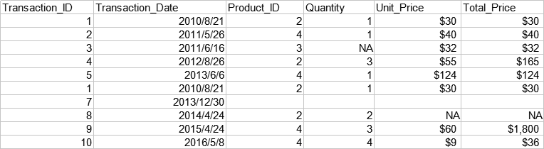
以下是一份简单的交易数据,包括交易单号,交易日期,产品序号,交易数量,单价,总价。
准备工作:导入pandas
import pandas as pd
读取数据: pd.read_excel(), pd.read_csv(), pd.read_json(), pd.read_sql(), pd.read_table()...
transactions=pd.read_excel(r'...\transactions.xlsx')
   Transaction_ID Transaction_Date Product_ID Quantity Unit_Price Total_Price

0               1       2010-08-21          2        1         30          30

1               2       2011-05-26          4        1         40          40

2               3       2011-06-16          3      NaN         32          32

3               4       2012-08-26          2        3         55         165

4               5       2013-06-06          4        1        124         124

5               1       2010-08-21          2        1         30          30

6               7       2013-12-30

7               8       2014-04-24          2        2        NaN         NaN

8               9       2015-04-24          4        3         60        1800

9              10       2016-05-08          4        4          9          36
获取数据信息:xx.info()
print(transactions.info())
RangeIndex: 10 entries, 0 to 9

Data columns (total 6 columns):

Transaction_ID      10 non-null int64

Transaction_Date    10 non-null datetime64[ns]

Product_ID          10 non-null object

Quantity            9 non-null object

Unit_Price          9 non-null object

Total_Price         9 non-null object

dtypes: datetime64[ns](1), int64(1), object(4)

memory usage: 560.0+ bytes

None
显示了数据各列的基本信息,比如:Transaction_ID有10个不为空的值,数据类型是int64; Quantity有9个不为空的值(说明有一个缺失值),数据类型是object;等等。
获取数据总行列数信息: xx.shape
print(transactions.shape)
(10, 6)
显示了数据共有10行6列。
获取所有行索引: xx.index.values
print(transactions.index.values)
[0 1 2 3 4 5 6 7 8 9]
获取所有列名: xx.columns.values
print(transactions.columns.values)
['Transaction_ID' 'Transaction_Date' 'Product_ID' 'Quantity' 'Unit_Price'

 'Total_Price']
选取某一行: xx.loc[row_index_name, : ] 显式 ; xx.iloc[row_index_from_zero, : ] 隐式
print(transactions.loc[1,:])
Transaction_ID                        2

Transaction_Date    2011-05-26 00:00:00

Product_ID                            4

Quantity                              1

Unit_Price                           40

Total_Price                          40

Name: 1, dtype: object
选取了数据的第二行。此数据行索引是从0开始一直到9,因此显式选取和隐式选取都一样。
选取某一列: xx['column_name']
print(transactions['Product_ID'])
0       2

1       4

2       3

3       2

4       4

5       2

6

7       2

8       4

9       4

Name: Product_ID, dtype: object
选取连续多行: xx.loc[row_index_name1: row_index_name2, : ] 显式 ; xx.iloc[row_index_from_zero1: row_index_from_zero2, : ] 隐式
print(transactions.iloc[2:4,:])
   Transaction_ID Transaction_Date Product_ID Quantity Unit_Price Total_Price

2               3       2011-06-16          3      NaN         32          32

3               4       2012-08-26          2        3         55         165
选取连续多列: xx.loc[ : , 'column_name1': 'column_name2'] 显式 ; xx.iloc[ : , column_index_from_zero1: column_index_from_zero2] 隐式
print(transactions.loc[:,'Product_ID':'Total_Price'])
  Product_ID Quantity Unit_Price Total_Price

0          2        1         30          30

1          4        1         40          40

2          3      NaN         32          32

3          2        3         55         165

4          4        1        124         124

5          2        1         30          30

6

7          2        2        NaN         NaN

8          4        3         60        1800

9          4        4          9          36
选取连续某几行某几列的数据: xx.loc[row_index_name1: row_index_name2, 'column_name1': 'column_name2'] 显式 ; xx.iloc[row_index_from_zero1: row_index_from_zero2, column_index_from_zero1: column_index_from_zero2] 隐式
print(transactions.iloc[2:4,2:4])
  Product_ID Quantity

2          3      NaN

3          2        3
选取不连续的多行: xx.loc[[row_index_name1,row_index_name2, ...], :] 显式 ; xx.iloc[[row_index_from_zero1, row_index_from_zero2, ...], :] 隐式
print(transactions.iloc[[1,4]])
   Transaction_ID Transaction_Date Product_ID Quantity Unit_Price Total_Price

1               2       2011-05-26          4        1         40          40

4               5       2013-06-06          4        1        124         124
选取不连续的多列: xx.loc[ :, [column_name1, column_name2, ...]] 显式 ; xx.iloc[ :, [column_index_from_zero1, column_index_from_zero2, ...]] 隐式
print(transactions.iloc[:,[1,4]])
  Transaction_Date Unit_Price

0       2010-08-21         30

1       2011-05-26         40

2       2011-06-16         32

3       2012-08-26         55

4       2013-06-06        124

5       2010-08-21         30

6       2013-12-30

7       2014-04-24        NaN

8       2015-04-24         60

9       2016-05-08          9
添加行: xx.loc[new_row_index]=[.....]
transactions.loc[10]=[11,"2018-9-9",1,4,2,8]
    Transaction_ID     Transaction_Date Product_ID Quantity Unit_Price  \

0                1  2010-08-21 00:00:00          2        1         30

1                2  2011-05-26 00:00:00          4        1         40

2                3  2011-06-16 00:00:00          3      NaN         32

3                4  2012-08-26 00:00:00          2        3         55

4                5  2013-06-06 00:00:00          4        1        124

5                1  2010-08-21 00:00:00          2        1         30

6                7  2013-12-30 00:00:00

7                8  2014-04-24 00:00:00          2        2        NaN

8                9  2015-04-24 00:00:00          4        3         60

9               10  2016-05-08 00:00:00          4        4          9

10              11             2018-9-9          1        4          2

   Total_Price

0           30

1           40

2           32

3          165

4          124

5           30

6

7          NaN

8         1800

9           36

10           8
添加列:xx['new_column_name']=[.....]
transactions['Unit_Profit']=[3,5,8,20,9,4,"",33,5,1]
   Transaction_ID Transaction_Date Product_ID Quantity Unit_Price Total_Price  \

0               1       2010-08-21          2        1         30          30

1               2       2011-05-26          4        1         40          40

2               3       2011-06-16          3      NaN         32          32

3               4       2012-08-26          2        3         55         165

4               5       2013-06-06          4        1        124         124

5               1       2010-08-21          2        1         30          30

6               7       2013-12-30

7               8       2014-04-24          2        2        NaN         NaN

8               9       2015-04-24          4        3         60        1800

9              10       2016-05-08          4        4          9          36

  Unit_Profit

0           3

1           5

2           8

3          20

4           9

5           4

6

7          33

8           5

9           1
在指定位置插入列: xx.insert(column_index, 'new_column_name',[...])
transactions.insert(5,'Unit_Profit',[3,5,8,20,9,4,"",33,5,1])
   Transaction_ID Transaction_Date Product_ID Quantity Unit_Price Unit_Profit  \

0               1       2010-08-21          2        1         30           3

1               2       2011-05-26          4        1         40           5

2               3       2011-06-16          3      NaN         32           8

3               4       2012-08-26          2        3         55          20

4               5       2013-06-06          4        1        124           9

5               1       2010-08-21          2        1         30           4

6               7       2013-12-30

7               8       2014-04-24          2        2        NaN          33

8               9       2015-04-24          4        3         60           5

9              10       2016-05-08          4        4          9           1

  Total_Price

0          30

1          40

2          32

3         165

4         124

5          30

6

7         NaN

8        1800

9          36
删除行:xx.drop(row_index_from_zero,axis=0)
transactions=transactions.drop(8,axis=0)
   Transaction_ID Transaction_Date Product_ID Quantity Unit_Price Total_Price

0               1       2010-08-21          2        1         30          30

1               2       2011-05-26          4        1         40          40

2               3       2011-06-16          3      NaN         32          32

3               4       2012-08-26          2        3         55         165

4               5       2013-06-06          4        1        124         124

5               1       2010-08-21          2        1         30          30

6               7       2013-12-30

7               8       2014-04-24          2        2        NaN         NaN

9              10       2016-05-08          4        4          9          36
删除列: xx.drop('column_name',axis=1)
transactions=transactions.drop('Total_Price',axis=1)
   Transaction_ID Transaction_Date Product_ID Quantity Unit_Price

0               1       2010-08-21          2        1         30

1               2       2011-05-26          4        1         40

2               3       2011-06-16          3      NaN         32

3               4       2012-08-26          2        3         55

4               5       2013-06-06          4        1        124

5               1       2010-08-21          2        1         30

6               7       2013-12-30

7               8       2014-04-24          2        2        NaN

8               9       2015-04-24          4        3         60

9              10       2016-05-08          4        4          9
数据转置: xx.T
print(transactions.T)
                                                          \

Transaction_ID

Transaction_Date  -- ::  -- ::

Product_ID

Quantity

Unit_Price

Total_Price

                                                          \

Transaction_ID

Transaction_Date  -- ::  -- ::

Product_ID

Quantity                          NaN

Unit_Price

Total_Price

                                                          \

Transaction_ID

Transaction_Date  -- ::  -- ::

Product_ID

Quantity

Unit_Price

Total_Price

                                                          \

Transaction_ID

Transaction_Date  -- ::  -- ::

Product_ID

Quantity

Unit_Price                                             NaN

Total_Price                                            NaN

Transaction_ID

Transaction_Date  -- ::  -- ::

Product_ID

Quantity

Unit_Price

Total_Price
有时候需要把行和列进行交换,数据才更容易看懂(尽管这里不需要)。
查找重复值: xx.duplicated()
print(transactions.duplicated())
0    False

1    False

2    False

3    False

4    False

5     True

6    False

7    False

8    False

9    False

dtype: bool
数据第6行(索引为5)是重复的(需要每列的数据都重复)。
删除重复值: xx.drop_duplicates()
transactions=transactions.drop_duplicates()
   Transaction_ID Transaction_Date Product_ID Quantity Unit_Price Total_Price

0               1       2010-08-21          2        1         30          30

1               2       2011-05-26          4        1         40          40

2               3       2011-06-16          3      NaN         32          32

3               4       2012-08-26          2        3         55         165

4               5       2013-06-06          4        1        124         124

6               7       2013-12-30

7               8       2014-04-24          2        2        NaN         NaN

8               9       2015-04-24          4        3         60        1800

9              10       2016-05-08          4        4          9          36
数据第6行已被删除。
查找缺失值: xx.isnull() ; xx.notnull()
print(transactions[transactions['Unit_Price'].isnull()])
   Transaction_ID Transaction_Date Product_ID Quantity Unit_Price Total_Price

7               8       2014-04-24          2        2        NaN         NaN
显示了Unit_Price有缺失值的一行数据。
删除缺失值: xx.dropna(how=..., axis=...) 注:how="any"或"all", axis=0或1
transactions=transactions.dropna(axis=0)
   Transaction_ID Transaction_Date Product_ID Quantity Unit_Price Total_Price

0               1       2010-08-21          2        1         30          30

1               2       2011-05-26          4        1         40          40

3               4       2012-08-26          2        3         55         165

4               5       2013-06-06          4        1        124         124

5               1       2010-08-21          2        1         30          30

6               7       2013-12-30

8               9       2015-04-24          4        3         60        1800

9              10       2016-05-08          4        4          9          36
填补缺失值: xx.fillna(value=..., axis=...) 注:axis=0或1
transactions['Unit_Price']=transactions['Unit_Price'].fillna(value=35)
   Transaction_ID Transaction_Date Product_ID Quantity Unit_Price Total_Price

0               1       2010-08-21          2        1         30          30

1               2       2011-05-26          4        1         40          40

2               3       2011-06-16          3      NaN         32          32

3               4       2012-08-26          2        3         55         165

4               5       2013-06-06          4        1        124         124

5               1       2010-08-21          2        1         30          30

6               7       2013-12-30

7               8       2014-04-24          2        2         35         NaN

8               9       2015-04-24          4        3         60        1800

9              10       2016-05-08          4        4          9          36
去除空格: 先把空格替换成NaN,再提取没有缺失值的数据
import numpy as np

transactions=transactions.applymap(lambda x: np.NaN if str(x).isspace() else x)
   Transaction_ID Transaction_Date  Product_ID  Quantity  Unit_Price  \

0               1       2010-08-21         2.0       1.0        30.0

1               2       2011-05-26         4.0       1.0        40.0

2               3       2011-06-16         3.0       NaN        32.0

3               4       2012-08-26         2.0       3.0        55.0

4               5       2013-06-06         4.0       1.0       124.0

5               1       2010-08-21         2.0       1.0        30.0

6               7       2013-12-30         NaN       NaN         NaN

7               8       2014-04-24         2.0       2.0         NaN

8               9       2015-04-24         4.0       3.0        60.0

9              10       2016-05-08         4.0       4.0         9.0

   Total_Price

0         30.0

1         40.0

2         32.0

3        165.0

4        124.0

5         30.0

6          NaN

7          NaN

8       1800.0

9         36.0
注:如果替换某行或某列的空格,用apply;如果替换整体数据的空格,则用applymap
转换数据类型:xx.astype(data_type_to_be_transferred_to) 注:可转换的数据类型有:int, str, float ... ; 转换成时间序列: pd.to_datetime(...)
transactions['Transaction_Date']=pd.to_datetime(transactions['Transaction_Date'])
注:需要先把数据内的缺失值处理干净,否则会产生错误
使用掩码进行条件筛选: xx[mask] 注:一些条件表示方法:&(and) ,|(or),~(not),.isin(in)
print(transactions[(transactions['Quantity']==1) & (transactions['Unit_Price']>100)])
   Transaction_ID Transaction_Date  Product_ID  Quantity  Unit_Price  \

4               5       2013-06-06         4.0       1.0       124.0

   Total_Price

4        124.0
这里选取了交易数量为1并且单价超过100的数据(删除了所有缺失值后)。
条件筛选后选取符合条件的某一列数据: xx.loc[xx[mask],'column_name']
print(transactions.loc[((transactions['Quantity']==1) & (transactions['Unit_Price']>100)),'Product_ID'])
4    4.0

Name: Product_ID, dtype: float64
这里选取了交易数量为1并且单价超过100的物品的Produxt_ID(删除了所有缺失值后)。
查找异常值: 通过掩码过滤,在这里以Upper Quartile+1.5*IQR和Lower Quartile-1.5*IQR为上下限
print(transactions.describe())

upper_extrme=144.5+1.5*(144.5-33)

lower_extrme=33-1.5*(144.5-33)

print(transactions.loc[((transactions['Total_Price']>upper_extrme) | (transactions['Total_Price']<lower_extrme))])
       Transaction_ID  Product_ID  Quantity  Unit_Price  Total_Price

count        7.000000    7.000000  7.000000    7.000000     7.000000

mean         4.571429    3.142857  2.000000   49.714286   317.857143

std          3.690399    1.069045  1.290994   36.926568   655.752095

min          1.000000    2.000000  1.000000    9.000000    30.000000

25%          1.500000    2.000000  1.000000   30.000000    33.000000

50%          4.000000    4.000000  1.000000   40.000000    40.000000

75%          7.000000    4.000000  3.000000   57.500000   144.500000

max         10.000000    4.000000  4.000000  124.000000  1800.000000

   Transaction_ID Transaction_Date  Product_ID  Quantity  Unit_Price  \

8               9       2015-04-24         4.0       3.0        60.0

   Total_Price

8       1800.0
先通过describe函数查看数据整体分布情况,然后计算出Total_Price的上下限,通过掩码选取Total_Price超过上限或低于下限的行。在这里可以看到,有一个异常值1800,原因是多写了一个0。
替换异常值: xx.replace(to_replace, new_value, inplace=True)
transactions['Total_Price'].replace(1800,180,inplace=True)
   Transaction_ID Transaction_Date  Product_ID  Quantity  Unit_Price  \

0               1       2010-08-21         2.0       1.0        30.0

1               2       2011-05-26         4.0       1.0        40.0

3               4       2012-08-26         2.0       3.0        55.0

4               5       2013-06-06         4.0       1.0       124.0

5               1       2010-08-21         2.0       1.0        30.0

8               9       2015-04-24         4.0       3.0        60.0

9              10       2016-05-08         4.0       4.0         9.0

   Total_Price

0         30.0

1         40.0

3        165.0

4        124.0

5         30.0

8        180.0

9         36.0
把上面查找出来的异常值1800替换成了180。
累计: 累计方法有:count(), mean(), median(), min(), max(), std(), prod(), sum(), ... 注:参数axis=0表示按行进行计算,axis=1表示按列进行计算,默认axis=1
print(transactions['Total_Price'].sum())
2225.0
显示了Total_Price的合计数目。
数据分组:xx.groupby(...)
print(transactions.groupby('Product_ID')['Quantity'].sum())
Product_ID

2.0    5.0

4.0    9.0

Name: Quantity, dtype: float64
显示了按照Product_ID分组的交易数量的总和。(注:transactions.groupby('Product_ID')是一个数据分组的对象,它实际上还没有进行任何计算,只是一个暂时存储的容器,要使用累计方法后才会进行计算。因此,groupby一般与累计函数搭配使用。)
如果需要对特定Series使用两个及以上的累计方法,请使用agg()。如果需要对整个DataFrame使用自定义的累计方法,请使用apply()。
print(transactions.groupby('Product_ID')['Quantity'].agg(['sum','mean']))
            sum      mean

Product_ID

2.0         5.0  1.666667

4.0         9.0  2.250000
计数: xx.value_counts()
print(transactions['Product_ID'].value_counts())
4.0    4

2.0    3

Name: Product_ID, dtype: int64
更改某个列名: xx.rename(columns={'old_column_name':'new_column_name'}, inplace=True)
transactions.rename(columns={'Unit_Price':'UP'},inplace=True)
   Transaction_ID Transaction_Date  Product_ID  Quantity     UP  Total_Price

0               1       2010-08-21         2.0       1.0   30.0         30.0

1               2       2011-05-26         4.0       1.0   40.0         40.0

3               4       2012-08-26         2.0       3.0   55.0        165.0

4               5       2013-06-06         4.0       1.0  124.0        124.0

5               1       2010-08-21         2.0       1.0   30.0         30.0

8               9       2015-04-24         4.0       3.0   60.0       1800.0

9              10       2016-05-08         4.0       4.0    9.0         36.0
批量更改列名:例如把所有列名中的下划线换成空格:xx.columns.str.replace('_', ' ')
更改索引: xx.set_index()
transactions.set_index('Transaction_Date',inplace=True)
                  Transaction_ID  Product_ID  Quantity  Unit_Price  \

Transaction_Date

2010-08-21                     1         2.0       1.0        30.0

2011-05-26                     2         4.0       1.0        40.0

2012-08-26                     4         2.0       3.0        55.0

2013-06-06                     5         4.0       1.0       124.0

2010-08-21                     1         2.0       1.0        30.0

2015-04-24                     9         4.0       3.0        60.0

2016-05-08                    10         4.0       4.0         9.0

                  Total_Price

Transaction_Date

2010-08-21               30.0

2011-05-26               40.0

2012-08-26              165.0

2013-06-06              124.0

2010-08-21               30.0

2015-04-24             1800.0

2016-05-08               36.0
以交易日期为索引。
按索引排序: xx.sort_index()
transactions.sort_index(ascending=False, inplace=True)
                  Transaction_ID  Product_ID  Quantity  Unit_Price  \

Transaction_Date

2016-05-08                    10         4.0       4.0         9.0

2015-04-24                     9         4.0       3.0        60.0

2013-06-06                     5         4.0       1.0       124.0

2012-08-26                     4         2.0       3.0        55.0

2011-05-26                     2         4.0       1.0        40.0

2010-08-21                     1         2.0       1.0        30.0

2010-08-21                     1         2.0       1.0        30.0

                  Total_Price

Transaction_Date

2016-05-08               36.0

2015-04-24             1800.0

2013-06-06              124.0

2012-08-26              165.0

2011-05-26               40.0

2010-08-21               30.0

2010-08-21               30.0
以交易日期为索引,倒序排列。
按内容排序: xx.sort_values()
transactions.sort_values(by=['Quantity','Total_Price'], inplace=True)
   Transaction_ID Transaction_Date  Product_ID  Quantity  Unit_Price  \

0               1       2010-08-21         2.0       1.0        30.0

5               1       2010-08-21         2.0       1.0        30.0

1               2       2011-05-26         4.0       1.0        40.0

4               5       2013-06-06         4.0       1.0       124.0

3               4       2012-08-26         2.0       3.0        55.0

8               9       2015-04-24         4.0       3.0        60.0

9              10       2016-05-08         4.0       4.0         9.0

   Total_Price

0         30.0

5         30.0

1         40.0

4        124.0

3        165.0

8       1800.0

9         36.0
更新索引: xx.reset_index()
transactions.reset_index(inplace=True)
   index  Transaction_ID Transaction_Date  Product_ID  Quantity  Unit_Price  \

0      0               1       2010-08-21         2.0       1.0        30.0

1      5               1       2010-08-21         2.0       1.0        30.0

2      1               2       2011-05-26         4.0       1.0        40.0

3      4               5       2013-06-06         4.0       1.0       124.0

4      3               4       2012-08-26         2.0       3.0        55.0

5      8               9       2015-04-24         4.0       3.0        60.0

6      9              10       2016-05-08         4.0       4.0         9.0

   Total_Price

0         30.0

1         30.0

2         40.0

3        124.0

4        165.0

5       1800.0

6         36.0
上面按内容排序后,索引顺序变乱了,如果数据就需要按此顺序排列,那么可以更新索引。
透视表: pd.pivot_table(xx, values=..., index=..., columns=..., aggfunc=...)
print(pd.pivot_table(transactions,values='Total_Price',index=['Product_ID','Quantity'],aggfunc='sum'))
                     Total_Price

Product_ID Quantity

2.0        1.0              60.0

           3.0             165.0

4.0        1.0             164.0

           3.0            1800.0

           4.0              36.0
多级索引行列转换: stack() ; unstack()
print(pd.pivot_table(transactions,values='Total_Price',index=['Product_ID','Quantity'],aggfunc='sum').unstack())
           Total_Price

Quantity           1.0     3.0   4.0

Product_ID

2.0               60.0   165.0   NaN

4.0              164.0  1800.0  36.0
将上面的透视表展开。
数据分列: xx.str.split()
假如我们要把交易日期里的年份提取出来,变成单独的列。---> 先把交易日期这一列的数据格式变为str,再按照'-'进行切割,当参数expand为True时,会把切割出来的内容分别当做一列。因此,如果只需要年份,那么就只需要提取第一列。
year=transactions['Transaction_Date'].astype(str).str.split('-',expand=True)[]

transactions['Year']=year
   Transaction_ID Transaction_Date  Product_ID  Quantity  Unit_Price  \

0               1       2010-08-21         2.0       1.0        30.0

1               2       2011-05-26         4.0       1.0        40.0

3               4       2012-08-26         2.0       3.0        55.0

4               5       2013-06-06         4.0       1.0       124.0

5               1       2010-08-21         2.0       1.0        30.0

8               9       2015-04-24         4.0       3.0        60.0

9              10       2016-05-08         4.0       4.0         9.0

   Total_Price  Year

0         30.0  2010

1         40.0  2011

3        165.0  2012

4        124.0  2013

5         30.0  2010

8       1800.0  2015

9         36.0  2016
这样,以后可以方便按年份或月份进行分组。
数据分区: pd.cut(xx, bins, labels=...) ; pd.qcut(xx, q, labels=...) 注:cut 是根据每个值的大小来进行分区的,qcut 是根据每个值出现的次数来进行分区的。
cut=pd.cut(transactions['Unit_Price'],3,labels=['low','median','high'])

transactions.insert(5,'Price_Range',cut)
   Transaction_ID Transaction_Date  Product_ID  Quantity  Unit_Price  \

0               1       2010-08-21         2.0       1.0        30.0

1               2       2011-05-26         4.0       1.0        40.0

3               4       2012-08-26         2.0       3.0        55.0

4               5       2013-06-06         4.0       1.0       124.0

5               1       2010-08-21         2.0       1.0        30.0

8               9       2015-04-24         4.0       3.0        60.0

9              10       2016-05-08         4.0       4.0         9.0

  Price_Range  Total_Price

0         low         30.0

1         low         40.0

3      median        165.0

4        high        124.0

5         low         30.0

8      median       1800.0

9         low         36.0
在这里把Unit_Price分成了3挡。
合并:
把列作为键进行合并: pd.merge(xx, xx, on=..., how=...)
假设我们现在有另外一张表,记载的是产品序号对应的产品名称。现在把这两张表合并在一起:
product_name=pd.DataFrame({"Product_ID":[1.0,2.0,3.0,4.0],"Product_Name":["candy","pen","stapler","toy"]})

merged=pd.merge(transactions,product_name,on='Product_ID',how="inner")
   Transaction_ID Transaction_Date  Product_ID  Quantity  Unit_Price  \

0               1       2010-08-21         2.0       1.0        30.0

1               4       2012-08-26         2.0       3.0        55.0

2               1       2010-08-21         2.0       1.0        30.0

3               2       2011-05-26         4.0       1.0        40.0

4               5       2013-06-06         4.0       1.0       124.0

5               9       2015-04-24         4.0       3.0        60.0

6              10       2016-05-08         4.0       4.0         9.0

   Total_Price Product_Name

0         30.0          pen

1        165.0          pen

2         30.0          pen

3         40.0          toy

4        124.0          toy

5       1800.0          toy

6         36.0          toy
假如两张表作为键的列名称不一致,那么可以通过设置left_on和left_on来解决:
product_name=pd.DataFrame({"Product_Identity":[1.0,2.0,3.0,4.0],"Product_Name":["candy","pen","stapler","toy"]})

merged=pd.merge(transactions,product_name,left_on='Product_ID',right_on="Product_Identity",how="inner")
   Transaction_ID Transaction_Date  Product_ID  Quantity  Unit_Price  \

0               1       2010-08-21         2.0       1.0        30.0

1               4       2012-08-26         2.0       3.0        55.0

2               1       2010-08-21         2.0       1.0        30.0

3               2       2011-05-26         4.0       1.0        40.0

4               5       2013-06-06         4.0       1.0       124.0

5               9       2015-04-24         4.0       3.0        60.0

6              10       2016-05-08         4.0       4.0         9.0

   Total_Price  Product_Identity Product_Name

0         30.0               2.0          pen

1        165.0               2.0          pen

2         30.0               2.0          pen

3         40.0               4.0          toy

4        124.0               4.0          toy

5       1800.0               4.0          toy

6         36.0               4.0          toy
注:how可选"left", "right", "outer", "inner"
"left":类似于SQL的left outer join;
"right":类似于SQL的right outer join;
"outer":并集,类似于SQL的full outer join;
"inner":交集,类似于SQL的inner join;
按索引进行合并: xx.join(xx, on=..., how=...)
假设有另外几张表(t1, t2)记载有交易记录,如果需要把这几张表合并在一起:transactions.join([t1,t2], how="outer")。这里不再做演示。
数据分析---用pandas进行数据清洗(Data Analysis Pandas Data Munging/Wrangling)的更多相关文章
- 用pandas进行数据清洗(二)(Data Analysis Pandas Data Munging/Wrangling)
在<用pandas进行数据清洗(一)(Data Analysis Pandas Data Munging/Wrangling)>中,我们介绍了数据清洗经常用到的一些pandas命令. 接下 ...
- Python For Data Analysis -- Pandas
首先pandas的作者就是这本书的作者 对于Numpy,我们处理的对象是矩阵 pandas是基于numpy进行封装的,pandas的处理对象是二维表(tabular, spreadsheet-like ...
- cookbook of python for data analysis
打算写讲义,目录已经想好. Content basic of python jupyter 开发环境 python 基本语法 利用python脚本完成工作 numpy for matrix compu ...
- How to use data analysis for machine learning (example, part 1)
In my last article, I stated that for practitioners (as opposed to theorists), the real prerequisite ...
- 《python for data analysis》第五章,pandas的基本使用
<利用python进行数据分析>一书的第五章源码与读书笔记 直接上代码 # -*- coding:utf-8 -*-# <python for data analysis>第五 ...
- 数据分析03 /基于pandas的数据清洗、级联、合并
数据分析03 /基于pandas的数据清洗.级联.合并 目录 数据分析03 /基于pandas的数据清洗.级联.合并 1. 处理丢失的数据 2. pandas处理空值操作 3. 数据清洗案例 4. 处 ...
- Python for Data Analysis 学习心得(二) - pandas介绍
一.pandas介绍 本篇程序上篇内容,在numpy下面继续介绍pandas,本书的作者是pandas的作者之一.pandas是非常好用的数据预处理工具,pandas下面有两个数据结构,分别为Seri ...
- pandas 之 数据清洗-缺失值
Abstract During the course fo doing data analysis and modeling, a significant amount of time is spen ...
- 数据分析---《Python for Data Analysis》学习笔记【04】
<Python for Data Analysis>一书由Wes Mckinney所著,中文译名是<利用Python进行数据分析>.这里记录一下学习过程,其中有些方法和书中不同 ...
随机推荐
- 2019 年起如何开始学习 ABP 框架系列文章-开篇有益
2019 年起如何开始学习 ABP 框架系列文章-开篇有益 [[TOC]] 本系列文章推荐阅读地址为:52ABP 开发文档 https://www.52abp.com/Wiki/52abp/lates ...
- 广播频道-BroadcastChannel
BroadcastChannel,就字面意思来言,叫做“广播频道”,官方文档说,该API是用于同源不同页面之间完成通信的功能. 1. 概况 它与window.postMessage的区别就是,Broa ...
- Truncated Power Method for Sparse Eigenvalue Problems
目录 算法 k的选择 \(x\)的初始化 代码 抱歉,真的没怎么看懂,当然,估计和我现在没法静下心来好好看也有关系. 算法 想法非常非常简单吧,就是在原来幂法的基础上,每次迭代的时候再加个截断.当然, ...
- 【RSYSLOG】Log4x To Rsyslog Config
Log4x To Rsyslog Config Log4net配置 <!--RemoteSyslogAppender--> <appender name="remoteSy ...
- ImageProcessor组件
ImageProcessor组件 开源免费的.NET图像即时处理的组件ImageProcessor 承接以前的组件系列,这个组件系列旨在介绍.NET相关的组件,让大家可以在项目中有一个更好的选择, ...
- html中怎么设置性别默认选择
<html><body> <form action="/example/html/form_action.asp" method="get& ...
- Individual Project
这次我自己完成了一个小小的项目,课可以把这篇随笔当做一次实验报告,主要的内容是用JUnit进行单元测试.由于我的技术太弱了,就在博客园里“求师”,按照大神的方法慢慢把这些东西写了下啦来. 不知道怎么搞 ...
- #Leetcode# 985. Sum of Even Numbers After Queries
https://leetcode.com/problems/sum-of-even-numbers-after-queries/ We have an array A of integers, and ...
- HowTos/Virtualization/VirtualBox - CentOS Wiki
https://wiki.centos.org/HowTos/Virtualization/VirtualBox
- Web系统大规模并发——秒杀与抢购 秒杀系统优化与预防措施
电商的秒杀和抢购,对我们来说,都不是一个陌生的东西.然而,从技术的角度来说,这对于Web系统是一个巨大的考验.当一个Web系统,在一秒钟内收到数以万计甚至更多请求时,系统的优化和稳定至关重要.这次我们 ...