(转)Polynomial interpolation 多项式插值

原文链接：https://blog.csdn.net/a19990412/article/details/87262531

 

扩展学习：https://www.sciencedirect.com/topics/mathematics/interpolation-polynomial

 

This example demonstrates how to approximate a function with a polynomial of degree n_degree by using ridge regression. Concretely, from n_samples 1d points, it suffices to build the Vandermonde matrix, which is n_samples x n_degree+1 and has the following form:

这个例子演示了如何用岭回归去近似一个函数用n_degree级的多项式级数。具体而言，从n_samples 1d个点，这满足去建立一个范德蒙德矩阵，有n_samples行，n_degree+1列。有如下的形式：

[[1,x1,x1∗∗2,x1∗∗3,…],[1,x2,x2∗∗2,x2∗∗3,…],…][[1,x1,x1∗∗2,x1∗∗3,…],[1,x2,x2∗∗2,x2∗∗3,…],…] [[1, x_1, x_1 ** 2, x_1 ** 3, …], \\ [1, x_2, x_2 ** 2, x_2 ** 3, …], …] [[1,x1​,x1​∗∗2,x1​∗∗3,…],[1,x2​,x2​∗∗2,x2​∗∗3,…],…]

Intuitively, this matrix can be interpreted as a matrix of pseudo features (the points raised to some power). The matrix is akin to (but different from) the matrix induced by a polynomial kernel.

直觉上来说，这个矩阵可以被理解为伪特征的矩阵。这些点提升到能量。
这个矩阵类似于（但不同于） 多项式核生成的矩阵。

This example shows that you can do non-linear regression with a linear model, using a pipeline to add non-linear features. Kernel methods extend this idea and can induce very high (even infinite) dimensional feature spaces.

这个例子显示，你可以用线性模型做非线性回归，通过管道来添加非线性特征。核方法扩展了这个想法，可以导出非常高维的（甚至是无限维）的特征空间。

实验过程

• 注意：
  • 这里是用高阶多项式来进行岭回归
  • 本质上不是我们日常所说的插值，因为插值点其实并不在对应的位置上。
  • 这里说的特征，在其实在fit之前只有一个多项式作为了特征。后面说到了这里采用的是岭回归。
    
    

# %pylab inline
# 如果是jupyter notebook就把上面一行注释去掉~
import numpy as np
import matplotlib.pyplot as plt

from sklearn.linear_model import Ridge
from sklearn.preprocessing import PolynomialFeatures
from sklearn.pipeline import make_pipeline

def f(x):
    """ function to approximate by polynomial interpolation"""
    return x * np.sin(x)

# generate points used to plot
x_plot = np.linspace(0, 10, 100)

# 随机获取20个插值点
# generate points and keep a subset of them
x = np.linspace(0, 10, 100) # 生成100个数据
rng = np.random.RandomState(0)
rng.shuffle(x)  # 随机打乱这个数据
x = np.sort(x[:20]) # 将前20个数据排序
y = f(x) #  放入f之中，获取散点的值

# create matrix versions of these arrays
X = x[:, np.newaxis]  # 将该数据提高一个维度
X_plot = x_plot[:, np.newaxis]  

colors = ['teal', 'yellowgreen', 'gold'] # 颜色集合
lw = 2  # 线宽度

# 真实数据所构成的曲线
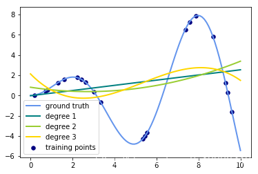
plt.plot(x_plot, f(x_plot), color='cornflowerblue', linewidth=lw,
         label="ground truth")

# 散点图，描出插值点
plt.scatter(x, y, color='navy', s=30, marker='o', label="training points")

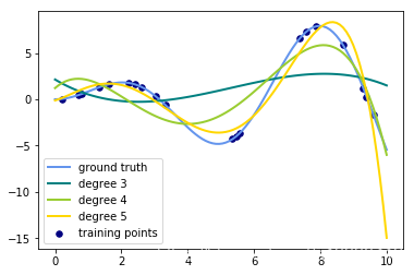
for count, degree in enumerate([3, 4, 5]):
    # 用degree的多项式特征结合上岭回归放入到管道之中构建模型
    model = make_pipeline(PolynomialFeatures(degree), Ridge())
#     print(model)
    model.fit(X, y)  # 训练模型
    y_plot = model.predict(X_plot) # 做出预测

    # 描绘出插值曲线
    plt.plot(x_plot, y_plot, color=colors[count], linewidth=lw,
             label="degree %d" % degree)

plt.legend(loc='lower left')
plt.show()

 

将for循环部分改成这样子：

for count, degree in enumerate([3]):
    # 用degree的多项式特征结合上岭回归放入到管道之中构建模型
    model = make_pipeline(PolynomialFeatures(degree), Ridge())
    model.fit(X, y)  # 训练模型
    y_plot = model.predict(X_plot) # 做出预测

    # 描绘出插值曲线
    plt.plot(x_plot, y_plot, color=colors[count], linewidth=lw,
             label="degree %d-Ridge" % degree)

    model = make_pipeline(PolynomialFeatures(degree), LinearRegression())
    model.fit(X, y)  # 训练模型
    y_plot = model.predict(X_plot) # 做出预测

    # 描绘出插值曲线
    plt.plot(x_plot, y_plot, color=colors[len(colors) - 1 - count], linewidth=lw,
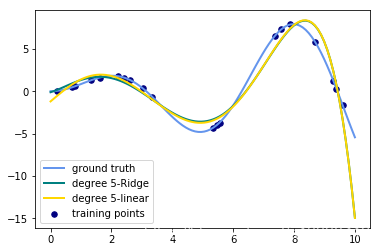
             label="degree %d-linear" % degree)

 

输出的图像为：(只需要将数值从3改成其他degree就可以生成其他图片了)

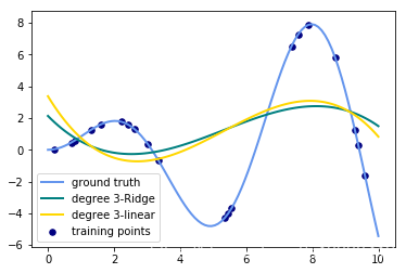
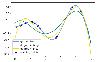
思考

• 观察：会发现岭回归的结果会线性回归的结果稍显波动小些。
• 回答：岭回归多加了一个L2的范数 约束了多项式特征的w的大小。