二、PyTorch 入门实战—Variable(转)
一、概念
1.Numpy里没有Variable这个概念,如果大家学过TensorFlow就会知道,Variable提供了自动求导的功能。
2.Variable需要放进一个计算图中,然后进行前后向传播和自动求导。
3.Variable的属性有三个:
- data:Variable里Tensor变量的数值
- grad:Variable反向传播的梯度
- grad_fn:得到Variable的操作
二、Variable的创建和使用
1.我们首先创建一个空的Variable:
import torch

#创建Variable

a = torch.autograd.Variable()

print(a)
结果如下:
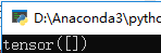
可以看到默认的类型为Tensor
2.那么,我们如果需要给Variable变量赋值,那么就一定是Tensor类型,例如:
b = torch.autograd.Variable(torch.Tensor([[1, 2], [3, 4],[5, 6], [7, 8]]))

print(b)
代码变为:
import torch
#创建Variable
a = torch.autograd.Variable()
print(a)
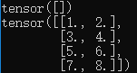
b = torch.autograd.Variable(torch.Tensor([[1, 2], [3, 4],[5, 6], [7, 8]]))
print(b)
结果为:
3.第一章提到了Variable的三个属性,我们依次打印它们:
import torch

#创建Variable

a = torch.autograd.Variable()

print(a)

b = torch.autograd.Variable(torch.Tensor([[1, 2], [3, 4],[5, 6], [7, 8]]))

print(b)

print(b.data)

print(b.grad)

print(b.grad_fn)
结果为:
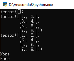
可以看到data就是Tensor的内容,剩下的两个属性为空
三、标量求导计算图
1.为了方便起见,我们可以将torch.autograd.Variable简写为Variable:
from torch.autograd import Variable
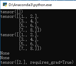
2.之后,我们先声明一个变量x,这里requires_grad=True意义是否对这个变量求梯度,默认的 Fa!se:
x = Variable(torch.Tensor([2]),requires_grad = True)

print(x)
代码变为:
import torch

#创建Variable

a = torch.autograd.Variable()

print(a)

b = torch.autograd.Variable(torch.Tensor([[1, 2], [3, 4],[5, 6], [7, 8]]))

print(b)

print(b.data)

print(b.grad)

print(b.grad_fn)

#建立计算图

from torch.autograd import Variable

x = Variable(torch.Tensor([2]),requires_grad = True)

print(x)
结果为:
3.我们再声明两个变量w和b:
w = Variable(torch.Tensor([3]),requires_grad = True)

print(w)

b = Variable(torch.Tensor([4]),requires_grad = True)

print(b)
4.我们再写两个变量y1和y2:
y1 = w * x + b

print(y1)

y2 = w * x + b * x

print(y2)
5.我们来计算各个变量的梯度,首先是y1:
#计算梯度

y1.backward()

print(x.grad)

print(w.grad)

print(b.grad)
代码变为:
import torch

#创建Variable

a = torch.autograd.Variable()

print(a)

b = torch.autograd.Variable(torch.Tensor([[1, 2], [3, 4],[5, 6], [7, 8]]))

print(b)

print(b.data)

print(b.grad)

print(b.grad_fn)

#建立计算图

from torch.autograd import Variable

x = Variable(torch.Tensor([2]),requires_grad = True)

print(x)

w = Variable(torch.Tensor([3]),requires_grad = True)

print(w)

b = Variable(torch.Tensor([4]),requires_grad = True)

print(b)

y1 = w * x + b

print(y1)

y2 = w * x + b * x

print(y2)

#计算梯度

y1.backward()

print(x.grad)

print(w.grad)

print(b.grad)
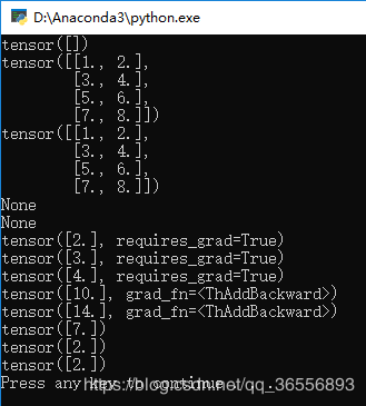
结果为:

其中:
y1 = 3 * 2 + 4 = 10,
y2 = 3 * 2 + 4 * 2 = 14,
x的梯度是3因为是3 * x,
w的梯度是2因为w * 2,
b的梯度是1因为b * 1(* 1被省略)
6.其次是y2,注销y1部分:
y2.backward(x)

print(x.grad)

print(w.grad)

print(b.grad)

代码为:

import torch

#创建Variable

a = torch.autograd.Variable()

print(a)

b = torch.autograd.Variable(torch.Tensor([[1, 2], [3, 4],[5, 6], [7, 8]]))

print(b)

print(b.data)

print(b.grad)

print(b.grad_fn)

#建立计算图

from torch.autograd import Variable

x = Variable(torch.Tensor([2]),requires_grad = True)

print(x)

w = Variable(torch.Tensor([3]),requires_grad = True)

print(w)

b = Variable(torch.Tensor([4]),requires_grad = True)

print(b)

y1 = w * x + b

print(y1)

y2 = w * x + b * x

print(y2)

#计算梯度

#y1.backward()

#print(x.grad)

#print(w.grad)

#print(b.grad)

y2.backward()

print(x.grad)

print(w.grad)

print(b.grad)
结果为:
其中:
x的梯度是7因为是3 * x + 4 * x,
w的梯度是2因为w * 2,
b的梯度是2因为b * 2
7.backward的函数可以填入参数,例如我们填入变量a:
a = Variable(torch.Tensor([5]),requires_grad = True)

y2.backward(a)

print(x.grad)

print(w.grad)

print(b.grad)
代码变为:
import torch

#创建Variable

a = torch.autograd.Variable()

print(a)

b = torch.autograd.Variable(torch.Tensor([[1, 2], [3, 4],[5, 6], [7, 8]]))

print(b)

print(b.data)

print(b.grad)

print(b.grad_fn)

#建立计算图

from torch.autograd import Variable

x = Variable(torch.Tensor([2]),requires_grad = True)

print(x)

w = Variable(torch.Tensor([3]),requires_grad = True)

print(w)

b = Variable(torch.Tensor([4]),requires_grad = True)

print(b)

y1 = w * x + b

print(y1)

y2 = w * x + b * x

print(y2)

#计算梯度

#y1.backward()

#print(x.grad)

#print(w.grad)

#print(b.grad)

a = Variable(torch.Tensor([5]),requires_grad = True)

y2.backward(a)

print(x.grad)

print(w.grad)

print(b.grad)
结果为:
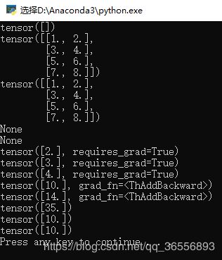
可以看到x,w,b的梯度乘以了a的值5,说明这个填入参数是梯度的系数。
四、矩阵求导计算图
1.例如:
#矩阵求导

c = torch.randn(3)

print(c)

c = Variable(c,requires_grad = True)

print(c)

y3 = c * 2

print(y3)

y3.backward(torch.FloatTensor([1, 0.1, 0.01]))

print(c.grad)
代码变为:
import torch

#创建Variable

a = torch.autograd.Variable()

print(a)

b = torch.autograd.Variable(torch.Tensor([[1, 2], [3, 4],[5, 6], [7, 8]]))

print(b)

print(b.data)

print(b.grad)

print(b.grad_fn)

#建立计算图

from torch.autograd import Variable

x = Variable(torch.Tensor([2]),requires_grad = True)

print(x)

w = Variable(torch.Tensor([3]),requires_grad = True)

print(w)

b = Variable(torch.Tensor([4]),requires_grad = True)

print(b)

y1 = w * x + b

print(y1)

y2 = w * x + b * x

print(y2)

#计算梯度

#y1.backward()

#print(x.grad)

#print(w.grad)

#print(b.grad)

a = Variable(torch.Tensor([5]),requires_grad = True)

y2.backward(a)

print(x.grad)

print(w.grad)

print(b.grad)

#矩阵求导

c = torch.randn(3)

print(c)

c = Variable(c,requires_grad = True)

print(c)

y3 = c * 2

print(y3)

y3.backward(torch.FloatTensor([1, 0.1, 0.01]))

print(c.grad)
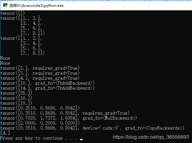
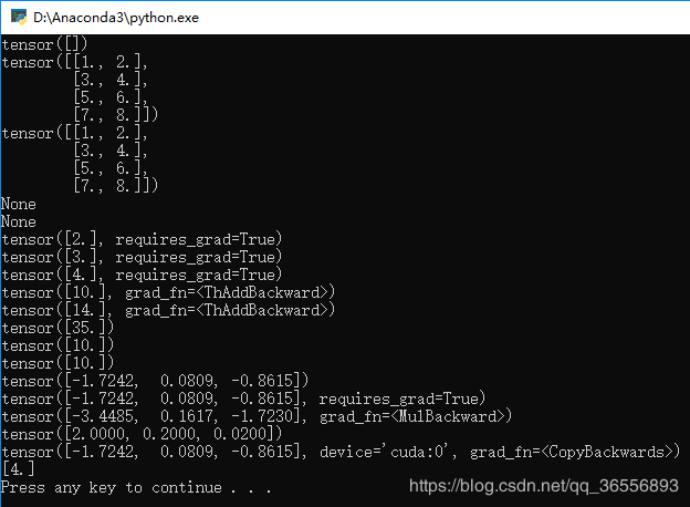
结果为:
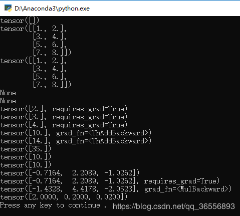
可以看到,c是一个1行3列的矩阵,因为y3 = c * 2,因此如果backward()里的参数为:
torch.FloatTensor([1, 1, 1])
则就是每个分量的梯度,但是传入的是:
torch.FloatTensor([1, 0.1, 0.01])
则每个分量梯度要分别乘以1,0.1和0.01
五、Variable放到GPU上执行
1.和Tensor一样的道理,代码如下:
#Variable放在GPU上

if torch.cuda.is_available():

d = c.cuda()

print(d)
代码变为:
import torch

#创建Variable

a = torch.autograd.Variable()

print(a)

b = torch.autograd.Variable(torch.Tensor([[1, 2], [3, 4],[5, 6], [7, 8]]))

print(b)

print(b.data)

print(b.grad)

print(b.grad_fn)

#建立计算图

from torch.autograd import Variable

x = Variable(torch.Tensor([2]),requires_grad = True)

print(x)

w = Variable(torch.Tensor([3]),requires_grad = True)

print(w)

b = Variable(torch.Tensor([4]),requires_grad = True)

print(b)

y1 = w * x + b

print(y1)

y2 = w * x + b * x

print(y2)

#计算梯度

#y1.backward()

#print(x.grad)

#print(w.grad)

#print(b.grad)

a = Variable(torch.Tensor([5]),requires_grad = True)

y2.backward(a)

print(x.grad)

print(w.grad)

print(b.grad)

#矩阵求导

c = torch.randn(3)

print(c)

c = Variable(c,requires_grad = True)

print(c)

y3 = c * 2

print(y3)

y3.backward(torch.FloatTensor([1, 0.1, 0.01]))

print(c.grad)

#Variable放在GPU上

if torch.cuda.is_available():

d = c.cuda()

print(d)
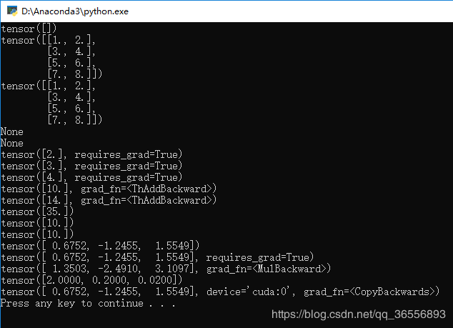
2.生成结果会慢一下,然后可以看到多了一个device=‘cuda:0’和grad_fn=<CopyBackwards>
六、Variable转Numpy与Numpy转Variable
1.值得注意的是,Variable里requires_grad 一般设置为 False,代码中为True则:
#变量转Numpy

e = Variable(torch.Tensor([4]),requires_grad = True)

f = e.numpy()

print(f)
会报如下错误:
Can't call numpy() on Variable that requires grad. Use var.detach().numpy() instead.
2.解决方法1:requires_grad改为False后,可以看到最后一行的Numpy类型的矩阵[4.]:
3.解决方法2::将numpy()改为detach().numpy(),可以看到最后一行的Numpy类型的矩阵[4.]
#变量转Numpy

e = Variable(torch.Tensor([4]),requires_grad = True)

f = e.detach().numpy()

print(f)
代码变为:
import torch

#创建Variable

a = torch.autograd.Variable()

print(a)

b = torch.autograd.Variable(torch.Tensor([[1, 2], [3, 4],[5, 6], [7, 8]]))

print(b)

print(b.data)

print(b.grad)

print(b.grad_fn)

#建立计算图

from torch.autograd import Variable

x = Variable(torch.Tensor([2]),requires_grad = True)

print(x)

w = Variable(torch.Tensor([3]),requires_grad = True)

print(w)

b = Variable(torch.Tensor([4]),requires_grad = True)

print(b)

y1 = w * x + b

print(y1)

y2 = w * x + b * x

print(y2)

#计算梯度

#y1.backward()

#print(x.grad)

#print(w.grad)

#print(b.grad)

a = Variable(torch.Tensor([5]),requires_grad = True)

y2.backward(a)

print(x.grad)

print(w.grad)

print(b.grad)

#矩阵求导

c = torch.randn(3)

print(c)

c = Variable(c,requires_grad = True)

print(c)

y3 = c * 2

print(y3)

y3.backward(torch.FloatTensor([1, 0.1, 0.01]))

print(c.grad)

#Variable放在GPU上

if torch.cuda.is_available():

d = c.cuda()

print(d)

#变量转Numpy

e = Variable(torch.Tensor([4]),requires_grad = True)

f = e.detach().numpy()

print(f)
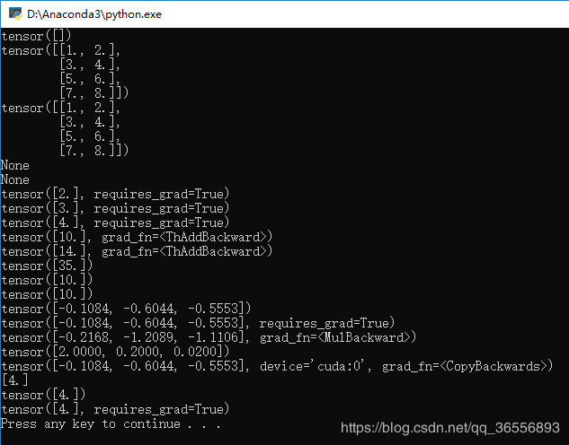
结果为:
4.Numpy转Variable先是转为Tensor再转为Variable:
#转换为Tensor

g = torch.from_numpy(f)

print(g)

#转换为Variable

g = Variable(g,requires_grad = True)

print(g)
代码变为:
import torch

#创建Variable

a = torch.autograd.Variable()

print(a)

b = torch.autograd.Variable(torch.Tensor([[1, 2], [3, 4],[5, 6], [7, 8]]))

print(b)

print(b.data)

print(b.grad)

print(b.grad_fn)

#建立计算图

from torch.autograd import Variable

x = Variable(torch.Tensor([2]),requires_grad = True)

print(x)

w = Variable(torch.Tensor([3]),requires_grad = True)

print(w)

b = Variable(torch.Tensor([4]),requires_grad = True)

print(b)

y1 = w * x + b

print(y1)

y2 = w * x + b * x

print(y2)

#计算梯度

#y1.backward()

#print(x.grad)

#print(w.grad)

#print(b.grad)

a = Variable(torch.Tensor([5]),requires_grad = True)

y2.backward(a)

print(x.grad)

print(w.grad)

print(b.grad)

#矩阵求导

c = torch.randn(3)

print(c)

c = Variable(c,requires_grad = True)

print(c)

y3 = c * 2

print(y3)

y3.backward(torch.FloatTensor([1, 0.1, 0.01]))

print(c.grad)

#Variable放在GPU上

if torch.cuda.is_available():

d = c.cuda()

print(d)

#变量转Numpy

e = Variable(torch.Tensor([4]),requires_grad = True)

f = e.detach().numpy()

print(f)

#转换为Tensor

g = torch.from_numpy(f)

print(g)

#转换为Variable

g = Variable(g,requires_grad = True)

print(g)
结果为:
七、Variable总结
1.Variable和Tensor本质上没有区别,不过Variable会被放入一个计算图中,然后进行前向传播,反向传播,自动求导。
2.Variable有三个属性,可以通过构造函数结构求取梯度得到grad值和grad_fn值
3.Variable,Tensor和Numpy互相转化很方便,类型也比较兼容
二、PyTorch 入门实战—Variable(转)的更多相关文章
- shiro实战系列(二)之入门实战续
下面讲解基于实战系列一,所以相关的java文件获取pom.xml及其log4j文件同样适用于本次讲解. 一.Using Shiro Using Shiro 现在我们的 SecurityManager ...
- 一、PyTorch 入门实战—Tensor(转)
目录 一.Tensor的创建和使用 二.Tensor放到GPU上执行 三.Tensor总结 一.Tensor的创建和使用 1.概念和TensorFlow的是基本一致的,只是代码编写格式的不同.我们声明 ...
- 深度学习入门实战(二)-用TensorFlow训练线性回归
欢迎大家关注腾讯云技术社区-博客园官方主页,我们将持续在博客园为大家推荐技术精品文章哦~ 作者 :董超 上一篇文章我们介绍了 MxNet 的安装,但 MxNet 有个缺点,那就是文档不太全,用起来可能 ...
- Pytorch入门——手把手教你MNIST手写数字识别
MNIST手写数字识别教程 要开始带组内的小朋友了,特意出一个Pytorch教程来指导一下 [!] 这里是实战教程,默认读者已经学会了部分深度学习原理,若有不懂的地方可以先停下来查查资料 目录 MNI ...
- Spark入门实战系列--2.Spark编译与部署(上)--基础环境搭建
[注] 1.该系列文章以及使用到安装包/测试数据 可以在<倾情大奉送--Spark入门实战系列>获取: 2.Spark编译与部署将以CentOS 64位操作系统为基础,主要是考虑到实际应用 ...
- Spark入门实战系列--6.SparkSQL(上)--SparkSQL简介
[注]该系列文章以及使用到安装包/测试数据 可以在<倾情大奉送--Spark入门实战系列>获取 .SparkSQL的发展历程 1.1 Hive and Shark SparkSQL的前身是 ...
- Spark入门实战系列--6.SparkSQL(下)--Spark实战应用
[注]该系列文章以及使用到安装包/测试数据 可以在<倾情大奉送--Spark入门实战系列>获取 .运行环境说明 1.1 硬软件环境 线程,主频2.2G,10G内存 l 虚拟软件:VMwa ...
- JMeter学习-004-WEB脚本入门实战
此文为 JMeter 入门实战实例.我是 JMeter 初学菜鸟一个,因而此文适合 JMeter 初学者参阅.同时,因本人知识有限,若文中存在不足的地方,敬请大神不吝指正,非常感谢! 闲话少述,话归正 ...
- webpack快速入门——实战技巧:优雅打包第三方类库
下面说两种方法: 一. 1.引入jQuery,首先安装: cnpm install --save jquery 2.安装好后,在我们的entry.js中引入: import $ from 'jquer ...
随机推荐
- Mybatis中的collection和association一关系
collection 一对多和association的多对一关系 学生和班级的一对多的例子 班级类: package com.glj.pojo; import java.io.Serializable ...
- Kafka 学习之路(一)—— Kafka简介
一.简介 Apache Kafka是一个分布式的流处理平台.它具有以下特点: 支持消息的发布和订阅,类似于RabbtMQ.ActiveMQ等消息队列: 支持数据实时处理: 能保证消息的可靠性投递: 支 ...
- ASP.NET Core[源码分析篇] - 认证
追本溯源,从使用开始 首先看一下我们的通常是如何使用微软自带的认证,一般在Startup里面配置我们所需的依赖认证服务,这里通过JWT的认证方式讲解 public void ConfigureServ ...
- Ruby中的常量:引号、%符号和heredoc
数值字面量 没什么好说的,唯一需要说明的是分数字面量:数值后加上一个后缀字母r表示分数字面量. # 整数字面量 0 1 100 10_000_001 # 千分位 # 浮点数字面量 0.1 1.0 1. ...
- Git 的一些使用细枝末节
新入职XX公司第一天, 使用旧同事的电脑 Step1: 在Android Studio 中配置帐号 $ git config --global user.name author #将用户名设为auth ...
- STL库的应用
容器分为两类:序列式容器和关联式容器. 序列式容器,其中的元素不一定有序,但都可以被排序.如:vector.list.deque.stack.queue.heap.priority_queue.sli ...
- netty实现的RPC框架
自己手撸了一个nettyRPC框架,希望在这里给有兴趣的同学们做个参考. 要想实现nettyrpc需要了解的技术要点如下: spring的自定义注解.spring的bean的有关初始化. 反射和动态代 ...
- Spring MVC源码(一) ----- 启动过程与组件初始化
SpringMVC作为MVC框架近年来被广泛地使用,其与Mybatis和Spring的组合,也成为许多公司开发web的套装.SpringMVC继承了Spring的优点,对业务代码的非侵入性,配置的便捷 ...
- Redis+Twemproxy分片存储实现
from unsplash 为提高Redis存储能力的提升,以及对外提供服务可用性提升,有时候有必要针对Redis进行集群式搭建,比较常用的有Twemproxy分片存储以及官方提供的Cluster方式 ...
- RabbitMQ(一):RabbitMQ快速入门
RabbitMQ是目前非常热门的一款消息中间件,不管是互联网大厂还是中小企业都在大量使用.作为一名合格的开发者,有必要对RabbitMQ有所了解,本文是RabbitMQ快速入门文章. RabbitMQ ...