使用scikit-learn解决文本多分类问题(附python演练)

来源 | TowardsDataScience

译者 | Revolver

在我们的商业世界中，存在着许多需要对文本进行分类的情况。例如，新闻报道通常按主题进行组织; 内容或产品通常需要按类别打上标签; 根据用户在线上谈论产品或品牌时的文字内容将用户分到不同的群组......

但是，互联网上的绝大多数文本分类文章和教程都是二文本分类，如垃圾邮件过滤（垃圾邮件与正常邮件），情感分析（正面与负面）。在大多数情况下，我们的现实世界问题要复杂得多。因此，这就是我们今天要做的事情：将消费者在金融方面的投诉分为12个事先定义好的类别。数据可以从data.gov

（https://catalog.data.gov/dataset/consumer-complaint-database）下载。

我们使用Python和Jupyter Notebook来开发我们的系统，并用到了Scikit-Learn中的机器学习组件。如果您想看到在PySpark

(https://medium.com/@actsusanli/multi-class-text-classification-with-pyspark-7d78d022ed35)上的实现，请阅读下一篇文章。

一、问题描述

我们的问题是是文本分类的有监督问题，我们的目标是调查哪种监督机器学习方法最适合解决它。

如果来了一条新的投诉，我们希望将其分配到12个类别中的一个。分类器假设每条新投诉都分配给一个且仅一个类别。这是文本多分类问题。是不是很迫不及待想看到我们可以做到什么程度呢！

二、数据探索

在深入研究机器学习模型之前，我们首先应该观察一下部分数据，看看每个类别下的投诉都是什么样儿？

import pandas as pd
df = pd.read_csv('Consumer_Complaints.csv')
df.head()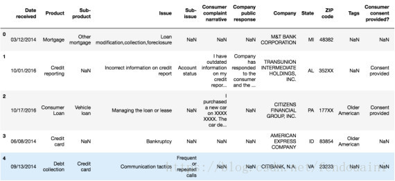

对于这个项目，我们其实只需要关注两列数据 - “Product”和“ Consumer complaint narrative ”（消费者投诉叙述）。

输入：Consumer_complaint_narrative

示例：“ I have outdated information on my credit report that I have previously disputed that has yet to be removed this information is more then seven years old and does not meet credit reporting requirements”

（“我的信用报告中存在过时信息，我之前已经提到过但还是没被删除， 此信息存在达七年之久，这并不符合信用报告要求”）

输出：Product

示例：Credit reporting （信用报告）

我们将移除“Consumer_complaint_narrative”这列中含缺失值的记录，并添加一列将Product编码为整数的列，因为分类标签通常更适合用整数表示而非字符串。

我们还创建了几个字典对象保存类标签和Product的映射关系，供将来使用。

清洗完毕后，以下是我们将要处理的前五行数据：

from io import StringIO
col = ['Product', 'Consumer complaint narrative']
df = df[col]
df = df[pd.notnull(df['Consumer complaint narrative'])]
df.columns = ['Product', 'Consumer_complaint_narrative']
df['category_id'] = df['Product'].factorize()[0]
category_id_df = df[['Product', 'category_id']].drop_duplicates().sort_values('category_id')
category_to_id = dict(category_id_df.values)
id_to_category = dict(category_id_df[['category_id', 'Product']].values)
df.head()

三、不平衡的类

我们发现每种产品收到的投诉记录的数量是不平衡的。消费者的投诉更倾向于Debt collection（债款收回），Credit reporting （信用报告），

Mortgage（抵押贷款。）

Import matplotlib.pyplot as plt
fig = plt.figure(figsize=(8,6))
df.groupby('Product').Consumer_complaint_narrative.count().plot.bar(ylim=0)
plt.show()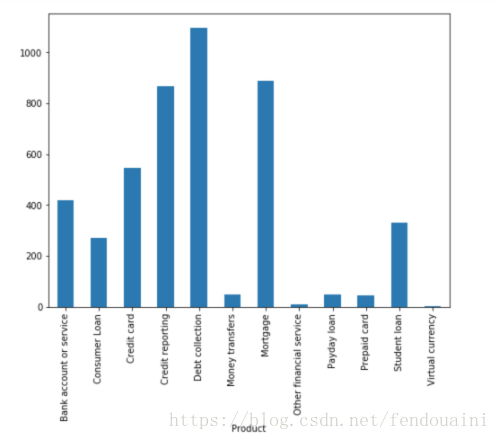

当我们遇到这样的问题时，如果用一般算法去解决问题就会遇到很多困难。传统算法通常不考虑数据分布，而倾向数量较大的类别。在最坏的情况下，少数群体会视为异常值被忽略。对于某些场景，例如欺诈检测或癌症预测，我们需要仔细配置我们的模型或人为地对数据集做再平衡处理，例如通过对每个类进行欠采样或过采样。

但是在我们今天这个例子里，数量多的类别正好可能是我们最感兴趣的部分。我们希望训练出这样一种分类器，该分类器在数量多的类别上提供高预测精度，同时又保持样本较少的类的合理准确性。因此，我们打算让数据集的比例保持原样，不做改变。

四、文本表示

分类器和学习算法没办法对文本的原始形式做直接处理，因为它们期望的输入是长度固定且为数值型的特征向量，而不是具有可变长度的原始文本。因此，在预处理阶段，文本需要被转换为更易于操作的表示形式。

从文本中提取特征的一种常用方法是使用词袋模型：对于每条文本样本，也即本案例中的Consumer_complaint_narrative，词袋模型会考虑单词的出现频率，但忽略它们出现的顺序。

具体来说，对于我们数据集中的每个单词，我们将计算它的词频和逆文档频率，简称tf-idf。我们将使用sklearn.feature_extraction.text.TfidfVectorizer 来计算每个消费者投诉叙述的向量的tf-idf向量：

（1） sublinear_df设置为True使用频率的对数形式。

（2） min_df 是一个单词必须存在的最小文档数量。

（3） norm设置为l2，以确保我们所有的特征向量是欧几里德范数为1的向量。

（4） ngram_range设置为(1, 2)表示我们要将文档的unigrams和bigrams两种形式的词条纳入我们的考虑。

（5） stop_words被设置为"english"删除所有诸如普通代词（"a"，"the"，...）的停用词，以减少噪音特征的数量。

from sklearn.feature_extraction.text import TfidfVectorizer
tfidf = TfidfVectorizer(sublinear_tf=True, min_df=5, norm='l2', encoding='latin-1', ngram_range=(1, 2), stop_words='english')
features = tfidf.fit_transform(df.Consumer_complaint_narrative).toarray()
labels = df.category_id
features.shape
（4569,12633）

现在，4569个消费者投诉叙述记录中的每一条都有12633个特征，代表不同的unigrams和bigrams的tf-idf分数。

我们可以用sklearn.feature_selection.chi2查找与每种类别（Product）最为相关的词条：

from sklearn.feature_selection import chi2
import numpy as np
N = 2
for Product, category_id in sorted(category_to_id.items()):
 features_chi2 = chi2(features, labels == category_id)
 indices = np.argsort(features_chi2[0])
 feature_names = np.array(tfidf.get_feature_names())[indices]
 unigrams = [v for v in feature_names if len(v.split(' ')) == 1]
 bigrams = [v for v in feature_names if len(v.split(' ')) == 2]
 print("# '{}':".format(Product))
 print("  . Most correlated unigrams:\n. {}".format('\n. '.join(unigrams[-N:])))
 print("  . Most correlated bigrams:\n. {}".format('\n. '.join(bigrams[-N:])))

# ‘Bank account or service’:
. Most correlated unigrams:
. bank
. overdraft
. Most correlated bigrams:
. overdraft fees
. checking account
# ‘Consumer Loan’:
. Most correlated unigrams:
. car
. vehicle
. Most correlated bigrams:
. vehicle xxxx
. toyota financial
# ‘Credit card’:
. Most correlated unigrams:
. citi
. card
. Most correlated bigrams:
. annual fee
. credit card
# ‘Credit reporting’:
. Most correlated unigrams:
. experian
. equifax
. Most correlated bigrams:
. trans union
. credit report
# ‘Debt collection’:
. Most correlated unigrams:
. collection
. debt
. Most correlated bigrams:
. collect debt
. collection agency
# ‘Money transfers’:
. Most correlated unigrams:
. wu
. paypal
. Most correlated bigrams:
. western union
. money transfer
# ‘Mortgage’:
. Most correlated unigrams:
. modification
. mortgage
. Most correlated bigrams:
. mortgage company
. loan modification

上面列出来的词条跟类别的匹配，看上去是不是好像有点道理？

五、多类标分类器：特征与设计

1. 为了训练有监督的分类器，我们首先将“Consumer_complaint_narrative”转变为数值向量。我们探索了诸如TF-IDF加权向量这样的向量表示。

2. 在文本有了自己的向量表示之后，我们就可以来训练有监督分类器模型，并对那些新来的“Consumer_complaint_narrative”预测它们所属的“Product”。

完成上述所有数据转换后，现在我们已经拥有了所有的特征和标签，现在是时候训练分类器了。我们可以使用许多算法来解决这类问题。

3. 朴素贝叶斯分类器：最适合单词统计的自然是朴素贝叶斯多项式模型：

from sklearn.model_selection import train_test_split
from sklearn.feature_extraction.text import CountVectorizer
from sklearn.feature_extraction.text import TfidfTransformer
from sklearn.naive_bayes import MultinomialNB
X_train, X_test, y_train, y_test = train_test_split(df['Consumer_complaint_narrative'], df['Product'], random_state = 0)
count_vect = CountVectorizer()
X_train_counts = count_vect.fit_transform(X_train)
tfidf_transformer = TfidfTransformer()
X_train_tfidf = tfidf_transformer.fit_transform(X_train_counts)
clf = MultinomialNB().fit(X_train_tfidf, y_train)

在对训练集训练之后，让我们用它来做一些预测。

print(clf.predict(count_vect.transform(["This company refuses to provide me verification and validation of debt per my right under the FDCPA. I do not believe this debt is mine."])))
[‘Debt collection’]

df[df['Consumer_complaint_narrative'] == "This company refuses to provide me verification and validation of debt per my right under the FDCPA. I do not believe this debt is mine."]

print(clf.predict(count_vect.transform(["I am disputing the inaccurate information the Chex-Systems has on my credit report. I initially submitted a police report on XXXX/XXXX/16 and Chex Systems only deleted the items that I mentioned in the letter and not all the items that were actually listed on the police report. In other words they wanted me to say word for word to them what items were fraudulent. The total disregard of the police report and what accounts that it states that are fraudulent. If they just had paid a little closer attention to the police report I would not been in this position now and they would n't have to research once again. I would like the reported information to be removed : XXXX XXXX XXXX"])))
[‘Credit reporting’]

df[df['Consumer_complaint_narrative'] == "I am disputing the inaccurate information the Chex-Systems has on my credit report. I initially submitted a police report on XXXX/XXXX/16 and Chex Systems only deleted the items that I mentioned in the letter and not all the items that were actually listed on the police report. In other words they wanted me to say word for word to them what items were fraudulent. The total disregard of the police report and what accounts that it states that are fraudulent. If they just had paid a little closer attention to the police report I would not been in this position now and they would n't have to research once again. I would like the reported information to be removed : XXXX XXXX XXXX"]
 

效果还不错！

六、模型选择

我们现在已经准备好尝试更多不同的机器学习模型，评估它们的准确性并找出任何潜在问题的根源。

我们将检测以下四种模型：

• 逻辑回归

• （多项式）朴素贝叶斯

• 线性支持向量机

• 随机森林

from sklearn.linear_model import LogisticRegression
from sklearn.ensemble import RandomForestClassifier
from sklearn.svm import LinearSVC
from sklearn.model_selection import cross_val_score
models = [
   RandomForestClassifier(n_estimators=200, max_depth=3, random_state=0),
   LinearSVC(),
   MultinomialNB(),
   LogisticRegression(random_state=0),
]
CV = 5
cv_df = pd.DataFrame(index=range(CV * len(models)))
entries = []
for model in models:
 model_name = model.__class__.__name__
 accuracies = cross_val_score(model, features, labels, scoring='accuracy', cv=CV)
 for fold_idx, accuracy in enumerate(accuracies):
   entries.append((model_name, fold_idx, accuracy))
cv_df = pd.DataFrame(entries, columns=['model_name', 'fold_idx', 'accuracy'])
import seaborn as sns
sns.boxplot(x='model_name', y='accuracy', data=cv_df)
sns.stripplot(x='model_name', y='accuracy', data=cv_df, 
             size=8, jitter=True, edgecolor="gray", linewidth=2)
plt.show()

cv_df.groupby('model_name').accuracy.mean()
model_name
LinearSVC: 0.822890
LogisticRegression: 0.792927
MultinomialNB: 0.688519
RandomForestClassifier: 0.443826
Name: accuracy, dtype: float64

线性支持向量机和逻辑回归比其他两个分类器表现更好，线性支持向量机略占优势，中值精度约为82%。

七、模型评估

接着继续探索我们的最佳模型（LinearSVC），先查看它混淆矩阵，然后显示预测值和实际标签之间的差异。

model = LinearSVC()
X_train, X_test, y_train, y_test, indices_train, indices_test = train_test_split(features, labels, df.index, test_size=0.33, random_state=0)
model.fit(X_train, y_train)
y_pred = model.predict(X_test)
from sklearn.metrics import confusion_matrix
conf_mat = confusion_matrix(y_test, y_pred)
fig, ax = plt.subplots(figsize=(10,10))
sns.heatmap(conf_mat, annot=True, fmt='d',
           xticklabels=category_id_df.Product.values, yticklabels=category_id_df.Product.values)
plt.ylabel('Actual')
plt.xlabel('Predicted')
plt.show()

预测结果的绝大多数都位于对角线上（预测标签=实际标签），也就是我们希望它们会落到的地方。但是还是存在不少错误的分类，找到错误的原因也是一件有意思的事情：

from IPython.display import display
for predicted in category_id_df.category_id:
 for actual in category_id_df.category_id:
   if predicted != actual and conf_mat[actual, predicted] >= 10:
     print("'{}' predicted as '{}' : {} examples.".format(id_to_category[actual], id_to_category[predicted], conf_mat[actual, predicted]))
     display(df.loc[indices_test[(y_test == actual) & (y_pred == predicted)]][['Product', 'Consumer_complaint_narrative']])
     print('')

正如您所看到的，一些错误分类的投诉往往涉及了多个主题（例如，同时涉及信用卡和信用报告两方面的投诉）。这种错误总会发生。

接着我们再一次使用卡方检验来查找与每个类别最相关的词条：

model.fit(features, labels)
N = 2
for Product, category_id in sorted(category_to_id.items()):
 indices = np.argsort(model.coef_[category_id])
 feature_names = np.array(tfidf.get_feature_names())[indices]
 unigrams = [v for v in reversed(feature_names) if len(v.split(' ')) == 1][:N]
 bigrams = [v for v in reversed(feature_names) if len(v.split(' ')) == 2][:N]
 print("# '{}':".format(Product))
 print("  . Top unigrams:\n       . {}".format('\n       . '.join(unigrams)))
 print("  . Top bigrams:\n       . {}".format('\n       . '.join(bigrams)))

# ‘Bank account or service’:
. Top unigrams:
. bank
. account
. Top bigrams:
. debit card
. overdraft fees
# ‘Consumer Loan’:
. Top unigrams:
. vehicle
. car
. Top bigrams:
. personal loan
. history xxxx
# ‘Credit card’:
. Top unigrams:
. card
. discover
. Top bigrams:
. credit card
. discover card
# ‘Credit reporting’:
. Top unigrams:
. equifax
. transunion
. Top bigrams:
. xxxx account
. trans union
# ‘Debt collection’:
. Top unigrams:
. debt
. collection
. Top bigrams:
. account credit
. time provided 

结果与我们的期望一致。

最后，我们打印出每个类别的分类报告：

from sklearn import metrics
print(metrics.classification_report(y_test, y_pred, target_names=df['Product'].unique()))

以上源代码（https://github.com/susanli2016/Machine-Learning-with-Python/blob/master/Consumer_complaints.ipynb）

都可以在Github上找到。