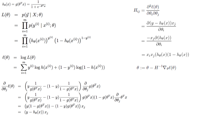
Logistic回归的牛顿法及DFP、BFGS拟牛顿法求解

牛顿法

  # coding:utf-8
 import matplotlib.pyplot as plt
 import numpy as np

 def dataN(length):#生成数据
     x = np.ones(shape = (length,3))
     y = np.zeros(length)
     for i in np.arange(0,length/100,0.02):
         x[100*i][0]=1
         x[100*i][1]=i
         x[100*i][2]=i + 1 + np.random.uniform(0,1.2)
         y[100*i]=1
         x[100*i+1][0]=1
         x[100*i+1][1]=i+0.01
         x[100*i+1][2]=i+0.01 + np.random.uniform(0,1.2)
         y[100*i+1]=0
     return x,y

 def sigmoid(x): #simoid 函数
     return 1.0/(1+np.exp(-x))

 def DFP(x,y, iter):#DFP拟牛顿法
     n = len(x[0])
     theta=np.ones((n,1))
     y=np.mat(y).T
     Gk=np.eye(n,n)
     grad_last = np.dot(x.T,sigmoid(np.dot(x,theta))-y)
     cost=[]
     for it in range(iter):
         pk = -1 * Gk.dot(grad_last)
         rate=alphA(x,y,theta,pk)
         theta = theta + rate * pk
         grad= np.dot(x.T,sigmoid(np.dot(x,theta))-y)
         delta_k = rate * pk
         y_k = (grad - grad_last)
         Pk = delta_k.dot(delta_k.T) / (delta_k.T.dot(y_k))
         Qk= Gk.dot(y_k).dot(y_k.T).dot(Gk) / (y_k.T.dot(Gk).dot(y_k)) * (-1)
         Gk += Pk + Qk
         grad_last = grad
         cost.append(np.sum(grad_last))
     return theta,cost

 def BFGS(x,y, iter):#BFGS拟牛顿法
     n = len(x[0])
     theta=np.ones((n,1))
     y=np.mat(y).T
     Bk=np.eye(n,n)
     grad_last = np.dot(x.T,sigmoid(np.dot(x,theta))-y)
     cost=[]
     for it in range(iter):
         pk = -1 * np.linalg.solve(Bk, grad_last)
         rate=alphA(x,y,theta,pk)
         theta = theta + rate * pk
         grad= np.dot(x.T,sigmoid(np.dot(x,theta))-y)
         delta_k = rate * pk
         y_k = (grad - grad_last)
         Pk = y_k.dot(y_k.T) / (y_k.T.dot(delta_k))
         Qk= Bk.dot(delta_k).dot(delta_k.T).dot(Bk) / (delta_k.T.dot(Bk).dot(delta_k)) * (-1)
         Bk += Pk + Qk
         grad_last = grad
         cost.append(np.sum(grad_last))
     return theta,cost

 def alphA(x,y,theta,pk): #选取前20次迭代cost最小的alpha
     c=float("inf")
     t=theta
     for k in range(1,200):
             a=1.0/k**2
             theta = t + a * pk
             f= np.sum(np.dot(x.T,sigmoid(np.dot(x,theta))-y))
             if abs(f)>c:
                 break
             c=abs(f)
             alpha=a
     return alpha

 def newtonMethod(x,y, iter):#牛顿法
     m = len(x)
     n = len(x[0])
     theta = np.zeros(n)
     cost=[]
     for it in range(iter):
         gradientSum = np.zeros(n)
         hessianMatSum = np.zeros(shape = (n,n))
         for i in range(m):
             hypothesis = sigmoid(np.dot(x[i], theta))
             loss =hypothesis-y[i]
             gradient = loss*x[i]
             gradientSum = gradientSum+gradient
             hessian=[b*x[i]*(1-hypothesis)*hypothesis for b in x[i]]
             hessianMatSum = np.add(hessianMatSum,hessian)
         hessianMatInv = np.mat(hessianMatSum).I
         for k in range(n):
             theta[k] -= np.dot(hessianMatInv[k], gradientSum)
         cost.append(np.sum(gradientSum))
     return theta,cost

 def tesT(theta, x, y):#准确率
     length=len(x)
     count=0
     for i in xrange(length):
         predict = sigmoid(x[i, :] * np.reshape(theta,(3,1)))[0] > 0.5
         if predict == bool(y[i]):
             count+= 1
     accuracy = float(count)/length
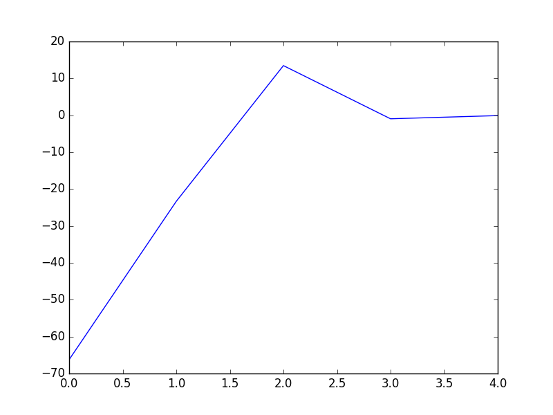
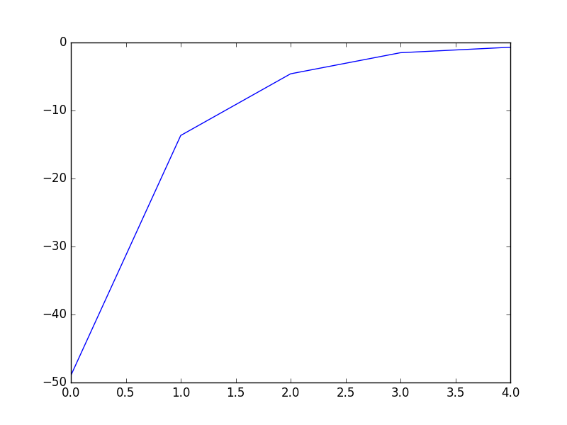
     return accuracy

 def showP(x,y,theta,cost,iter):#作图
     plt.figure(1)
     plt.plot(range(iter),cost)
     plt.figure(2)
     color=['or','ob']
     for i in xrange(length):
         plt.plot(x[i, 1], x[i, 2],color[int(y[i])])
     plt.plot([0,length/100],[-theta[0],-theta[0]-theta[1]*length/100]/theta[2])
     plt.show()
 length=200
 iter=5
 x,y=dataN(length)

 theta,cost=BFGS(x,y,iter)
 print theta   #[[-18.93768161][-16.52178427][ 16.95779981]]
 print tesT(theta, np.mat(x), y)  #0.935
 showP(x,y,theta.getA(),cost,iter)

 theta,cost=DFP(x,y,iter)
 print theta   #[[-18.51841028][-16.17880599][ 16.59649161]]
 print tesT(theta, np.mat(x), y)  #0.935
 showP(x,y,theta.getA(),cost,iter)

 theta,cost=newtonMethod(x,y,iter)
 print theta   #[-14.49650536 -12.78692552  13.05843361]
 print tesT(theta, np.mat(x), y)  #0.935
 showP(x,y,theta,cost,iter)