BAYESIAN STATISTICS AND CLINICAL TRIAL CONCLUSIONS: WHY THE OPTIMSE STUDY SHOULD BE CONSIDERED POSITIVE（转）

Statistical approaches to randomised controlled trial analysis

The statistical approach used in the design and analysis of the vast majority of clinical studies is often referred to as classical or frequentist. Conclusions are made on the results of hypothesis tests with generation of p-values and confidence intervals, and require that the correct conclusion be drawn with a high probability among a notional set of repetitions of the trial.

Bayesian inference is an alternative, which treats conclusions probabilistically and provides a different framework for thinking about trial design and conclusions. There are many differences between the two, but for this discussion there are two obvious distinctions with the Bayesian approach. The first is that prior knowledge can be accounted for to a greater or lesser extent, something life scientists sometimes have difficulty reconciling. Secondly, the conclusions of a Bayesian analysis often focus on the decision that requires to be made, e.g. should this new treatment be used or not.

There are pros and cons to both sides, nicely discussed here, but I would argue that the results of frequentist analyses are too often accepted with insufficient criticism. Here’s a good example.

OPTIMSE: Optimisation of Cardiovascular Management to Improve Surgical Outcome

Optimising the amount of blood being pumped out of the heart during surgery may improve patient outcomes. By specifically measuring cardiac output in the operating theatre and using it to guide intravenous fluid administration and the use of drugs acting on the circulation, the amount of oxygen that is delivered to tissues can be increased.

It sounds like common sense that this would be a good thing, but drugs can have negative effects, as can giving too much intravenous fluid. There are also costs involved, is the effort worth it? Small trials have suggested that cardiac output-guided therapy may have benefits, but the conclusion of a large Cochrane review was that the results remain uncertain.

A well designed and run multi-centre randomised controlled trial was performed to try and determine if this intervention was of benefit (OPTIMSE: Optimisation of Cardiovascular Management to Improve Surgical Outcome).

Patients were randomised to a cardiac output–guided hemodynamic therapy algorithm for intravenous fluid and a drug to increase heart muscle contraction (the inotrope, dopexamine) during and 6 hours following surgery (intervention group) or to usual care (control group).

The primary outcome measure was the relative risk (RR) of a composite of 30-day moderate or major complications and mortality.

OPTIMSE: reported results

Focusing on the primary outcome measure, there were 158/364 (43.3%) and 134/366 (36.6%) patients with complication/mortality in the control and intervention group respectively. Numerically at least, the results appear better in the intervention group compared with controls.

Using the standard statistical approach, the relative risk (95% confidence interval) = 0.84 (0.70-1.01), p=0.07 and absolute risk difference = 6.8% (−0.3% to 13.9%), p=0.07. This is interpreted as there being insufficient evidence that the relative risk for complication/death is different to 1.0 (all analyses replicated below). The authors reasonably concluded that:

In a randomized trial of high-risk patients undergoing major gastrointestinal surgery, use of a cardiac output–guided hemodynamic therapy algorithm compared with usual care did not reduce a composite outcome of complications and 30-day mortality.

A difference does exist between the groups, but is not judged to be a sufficient difference using this conventional approach.

OPTIMSE: Bayesian analysis

Repeating the same analysis using Bayesian inference provides an alternative way to think about this result. What are the chances the two groups actually do have different results? What are the chances that the two groups have clinically meaningful differences in results? What proportion of patients stand to benefit from the new intervention compared with usual care?

With regard to prior knowledge, this analysis will not presume any prior information. This makes the point that prior information is not always necessary to draw a robust conclusion. It may be very reasonable to use results from pre-existing meta-analyses to specify a weak prior, but this has not been done here. Very grateful to John Kruschke for the excellent scripts and book, Doing Bayesian Data Analysis.

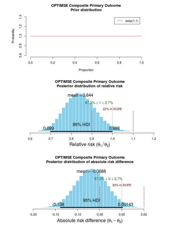
The results of the analysis are presented in the graph below. The top panel is the prior distribution. All proportions for the composite outcome in both the control and intervention group are treated as equally likely.

The middle panel contains the main findings. This is the posterior distribution generated in the analysis for the relative risk of the composite primary outcome (technical details in script below).

The mean relative risk = 0.84 which as expected is the same as the frequentist analysis above. Rather than confidence intervals, in Bayesian statistics a credible interval or region is quoted (HDI = highest density interval is the same). This is philosphically different to a confidence interval and says:

Given the observed data, there is a 95% probability that the true RR falls within this credible interval.

This is a subtle distinction to the frequentist interpretation of a confidence interval:

Were I to repeat this trial multiple times and compute confidence intervals, there is a 95% probability that the true RR would fall within these confidence intervals.

This is an important distinction and can be extended to make useful probabilistic statements about the result.

The figures in green give us the proportion of the distribution above and below 1.0. We can therefore say:

The probability that the intervention group has a lower incidence of the composite endpoint is 97.3%.

It may be useful to be more specific about the size of difference between the control and treatment group that would be considered equivalent, e.g. 10% above and below a relative risk = 1.0. This is sometimes called the region of practical equivalence (ROPE; red text on plots). Experts would determine what was considered equivalent based on many factors. We could therefore say:

The probability of the composite end-point for the control and intervention group being equivalent is 22%.

Or, the probability of a clinically relevant difference existing in the composite endpoint between control and intervention groups is 78%

Finally, we can use the 200 000 estimates of the probability of complication/death in the control and intervention groups that were generated in the analysis (posterior prediction). In essence, we can act like these are 2 x 200 000 patients. For each “patient pair”, we can use their probability estimates and perform a random draw to simulate the occurrence of complication/death. It may be useful then to look at the proportion of “patients pairs” where the intervention patient didn’t have a complication but the control patient did:

Using posterior prediction on the generated Bayesian model, the probability that a patient in the intervention group did not have a complication/death when a patient in the control group did have a complication/death is 28%.

Conclusion

On the basis of a standard statistical analysis, the OPTIMISE trial authors reasonably concluded that the use of the intervention compared with usual care did not reduce a composite outcome of complications and 30-day mortality.

Using a Bayesian approach, it could be concluded with 97.3% certainty that use of the intervention compared with usual care reduces the composite outcome of complications and 30-day mortality; that with 78% certainty, this reduction is clinically significant; and that in 28% of patients where the intervention is used rather than usual care, complication or death may be avoided.

 # OPTIMISE trial in a Bayesian framework

 # JAMA. 2014;311(21):2181-2190. doi:10.1001/jama.2014.5305

 # Ewen Harrison

 # 15/02/2015

 # Primary outcome: composite of 30-day moderate or major complications and mortality

 N1 <- 366

 y1 <- 134

 N2 <- 364

 y2 <- 158

 # N1 is total number in the Cardiac Output–Guided Hemodynamic Therapy Algorithm (intervention) group

 # y1 is number with the outcome in the Cardiac Output–Guided Hemodynamic Therapy Algorithm (intervention) group

 # N2 is total number in usual care (control) group

 # y2 is number with the outcome in usual care (control) group

 # Risk ratio

 (y1/N1)/(y2/N2)

 library(epitools)

 riskratio(c(N1-y1, y1, N2-y2, y2), rev="rows", method="boot", replicates=100000)

 # Using standard frequentist approach

 # Risk ratio (bootstrapped 95% confidence intervals) = 0.84 (0.70-1.01)

 # p=0.07 (Fisher exact p-value)

 # Reasonably reported as no difference between groups.

 # But there is a difference, it just not judged significant using conventional

 # (and much criticised) wisdom.

 # Bayesian analysis of same ratio

 # Base script from John Krushcke, Doing Bayesian Analysis

 #------------------------------------------------------------------------------

 source("~/Doing_Bayesian_Analysis/openGraphSaveGraph.R")

 source("~/Doing_Bayesian_Analysis/plotPost.R")

 require(rjags) # Kruschke, J. K. (2011). Doing Bayesian Data Analysis, Academic Press / Elsevier.

 #------------------------------------------------------------------------------

 # Important

 # The model will be specified with completely uninformative prior distributions (beta(1,1,).

 # This presupposes that no pre-exisiting knowledge exists as to whehther a difference

 # may of may not exist between these two intervention.

 # Plot Beta(1,1)

 # 3x1 plots

 par(mfrow=c(3,1))

 # Adjust size of prior plot

 par(mar=c(5.1,7,4.1,7))

 plot(seq(0, 1, length.out=100), dbeta(seq(0, 1, length.out=100), 1, 1),

 type="l", xlab="Proportion",

 ylab="Probability",

 main="OPTIMSE Composite Primary Outcome\nPrior distribution",

 frame=FALSE, col="red", oma=c(6,6,6,6))

 legend("topright", legend="beta(1,1)", lty=1, col="red", inset=0.05)

 # THE MODEL.

 modelString = "

 # JAGS model specification begins here...

 model {

 # Likelihood. Each complication/death is Bernoulli.

 for ( i in 1 : N1 ) { y1[i] ~ dbern( theta1 ) }

 for ( i in 1 : N2 ) { y2[i] ~ dbern( theta2 ) }

 # Prior. Independent beta distributions.

 theta1 ~ dbeta( 1 , 1 )

 theta2 ~ dbeta( 1 , 1 )

 }

 # ... end JAGS model specification

 " # close quote for modelstring

 # Write the modelString to a file, using R commands:

 writeLines(modelString,con="model.txt")

 #------------------------------------------------------------------------------

 # THE DATA.

 # Specify the data in a form that is compatible with JAGS model, as a list:

 dataList = list(

 N1 = N1 ,

 y1 = c(rep(1, y1), rep(0, N1-y1)),

 N2 = N2 ,

 y2 = c(rep(1, y2), rep(0, N2-y2))

 )

 #------------------------------------------------------------------------------

 # INTIALIZE THE CHAIN.

 # Can be done automatically in jags.model() by commenting out inits argument.

 # Otherwise could be established as:

 # initsList = list( theta1 = sum(dataList$y1)/length(dataList$y1) ,

 #                   theta2 = sum(dataList$y2)/length(dataList$y2) )

 #------------------------------------------------------------------------------

 # RUN THE CHAINS.

 parameters = c( "theta1" , "theta2" )     # The parameter(s) to be monitored.

 adaptSteps = 500              # Number of steps to "tune" the samplers.

 burnInSteps = 1000            # Number of steps to "burn-in" the samplers.

 nChains = 3                   # Number of chains to run.

 numSavedSteps=200000           # Total number of steps in chains to save.

 thinSteps=1                   # Number of steps to "thin" (1=keep every step).

 nIter = ceiling( ( numSavedSteps * thinSteps ) / nChains ) # Steps per chain.

 # Create, initialize, and adapt the model:

 jagsModel = jags.model( "model.txt" , data=dataList , # inits=initsList ,

 n.chains=nChains , n.adapt=adaptSteps )

 # Burn-in:

 cat( "Burning in the MCMC chain...\n" )

 update( jagsModel , n.iter=burnInSteps )

 # The saved MCMC chain:

 cat( "Sampling final MCMC chain...\n" )

 codaSamples = coda.samples( jagsModel , variable.names=parameters ,

 n.iter=nIter , thin=thinSteps )

 # resulting codaSamples object has these indices:

 #   codaSamples[[ chainIdx ]][ stepIdx , paramIdx ]

 #------------------------------------------------------------------------------

 # EXAMINE THE RESULTS.

 # Convert coda-object codaSamples to matrix object for easier handling.

 # But note that this concatenates the different chains into one long chain.

 # Result is mcmcChain[ stepIdx , paramIdx ]

 mcmcChain = as.matrix( codaSamples )

 theta1Sample = mcmcChain[,"theta1"] # Put sampled values in a vector.

 theta2Sample = mcmcChain[,"theta2"] # Put sampled values in a vector.

 # Plot the chains (trajectory of the last 500 sampled values).

 par( pty="s" )

 chainlength=NROW(mcmcChain)

 plot( theta1Sample[(chainlength-500):chainlength] ,

 theta2Sample[(chainlength-500):chainlength] , type = "o" ,

 xlim = c(0,1) , xlab = bquote(theta[1]) , ylim = c(0,1) ,

 ylab = bquote(theta[2]) , main="JAGS Result" , col="skyblue" )

 # Display means in plot.

 theta1mean = mean(theta1Sample)

 theta2mean = mean(theta2Sample)

 if (theta1mean > .5) { xpos = 0.0 ; xadj = 0.0

 } else { xpos = 1.0 ; xadj = 1.0 }

 if (theta2mean > .5) { ypos = 0.0 ; yadj = 0.0

 } else { ypos = 1.0 ; yadj = 1.0 }

 text( xpos , ypos ,

 bquote(

 "M=" * .(signif(theta1mean,3)) * "," * .(signif(theta2mean,3))

 ) ,adj=c(xadj,yadj) ,cex=1.5  )

 # Plot a histogram of the posterior differences of theta values.

 thetaRR = theta1Sample / theta2Sample # Relative risk

 thetaDiff = theta1Sample - theta2Sample # Absolute risk difference

 par(mar=c(5.1, 4.1, 4.1, 2.1))

 plotPost( thetaRR , xlab= expression(paste("Relative risk (", theta[1]/theta[2], ")")) ,

 compVal=1.0, ROPE=c(0.9, 1.1),

 main="OPTIMSE Composite Primary Outcome\nPosterior distribution of relative risk")

 plotPost( thetaDiff , xlab=expression(paste("Absolute risk difference (", theta[1]-theta[2], ")")) ,

 compVal=0.0, ROPE=c(-0.05, 0.05),

 main="OPTIMSE Composite Primary Outcome\nPosterior distribution of absolute risk difference")

 #-----------------------------------------------------------------------------

 # Use posterior prediction to determine proportion of cases in which

 # using the intervention would result in no complication/death

 # while not using the intervention would result in complication death

 chainLength = length( theta1Sample )

 # Create matrix to hold results of simulated patients:

 yPred = matrix( NA , nrow=2 , ncol=chainLength )

 # For each step in chain, use posterior prediction to determine outcome

 for ( stepIdx in 1:chainLength ) { # step through the chain

 # Probability for complication/death for each "patient" in intervention group:

 pDeath1 = theta1Sample[stepIdx]

 # Simulated outcome for each intervention "patient"

 yPred[1,stepIdx] = sample( x=c(0,1), prob=c(1-pDeath1,pDeath1), size=1 )

 # Probability for complication/death for each "patient" in control group:

 pDeath2 = theta2Sample[stepIdx]

 # Simulated outcome for each control "patient"

 yPred[2,stepIdx] = sample( x=c(0,1), prob=c(1-pDeath2,pDeath2), size=1 )

 }

 # Now determine the proportion of times that the intervention group has no complication/death

 # (y1 == 0) and the control group does have a complication or death (y2 == 1))

 (pY1eq0andY2eq1 = sum( yPred[1,]==0 & yPred[2,]==1 ) / chainLength)

 (pY1eq1andY2eq0 = sum( yPred[1,]==1 & yPred[2,]==0 ) / chainLength)

 (pY1eq0andY2eq0 = sum( yPred[1,]==0 & yPred[2,]==0 ) / chainLength)

 (pY10eq1andY2eq1 = sum( yPred[1,]==1 & yPred[2,]==1 ) / chainLength)

 # Conclusion: in 27% of cases based on these probabilities,

 # a patient in the intervention group would not have a complication,

 # when a patient in control group did.

转自：http://www.datasurg.net/2015/02/16/bayesian-statistics-and-clinical-trial-conclusions-why-the-optimse-study-should-be-considered-positive/