转载 Deep learning：六(regularized logistic回归练习)

前言：

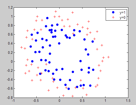
在上一讲Deep learning：五(regularized线性回归练习)中已经介绍了regularization项在线性回归问题中的应用，这节主要是练习regularization项在logistic回归中的应用，并使用牛顿法来求解模型的参数。参考的网页资料为：http://openclassroom.stanford.edu/MainFolder/DocumentPage.php?course=DeepLearning&doc=exercises/ex5/ex5.html。要解决的问题是，给出了具有2个特征的一堆训练数据集，从该数据的分布可以看出它们并不是非常线性可分的，因此很有必要用更高阶的特征来模拟。例如本程序中个就用到了特征值的6次方来求解。

实验基础：

contour:

该函数是绘制轮廓线的，比如程序中的contour(u, v, z, [0, 0], 'LineWidth', 2)，指的是在二维平面U-V中绘制曲面z的轮廓，z的值为0，轮廓线宽为2。注意此时的z对应的范围应该与U和V所表达的范围相同。因为contour函数是用来等高线，而本实验中只需画一条等高线，所以第4个参数里面的值都是一样的，这里为[0,0],0指的是函数值z在0和0之间的等高线(很明显，只能是一条)。

在logistic回归中，其表达式为：

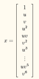
在此问题中，将特征x映射到一个28维的空间中，其x向量映射后为：

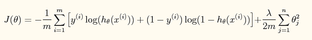
此时加入了规则项后的系统的损失函数为：

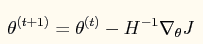
对应的牛顿法参数更新方程为：

其中：

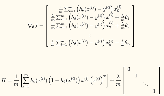
公式中的一些宏观说明（直接截的原网页）：

实验结果：

原训练数据点的分布情况：

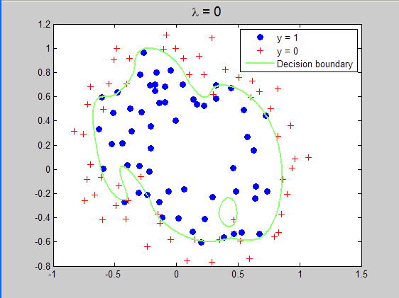
当lambda=0时所求得的分界曲面：

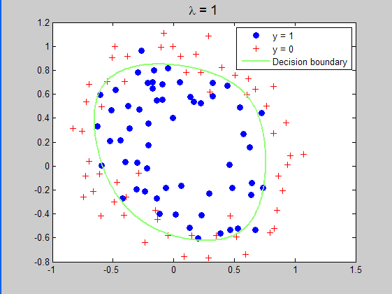
当lambda=1时所求得的分界曲面：

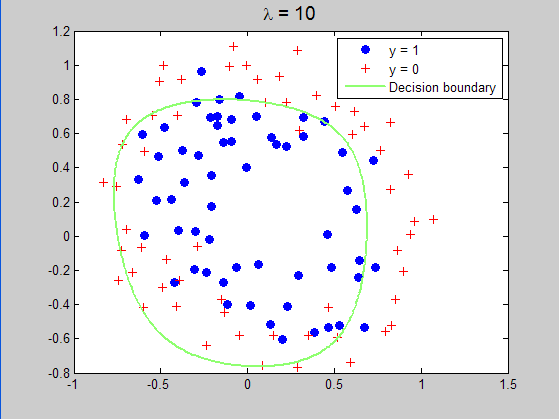
当lambda=10时所求得的分界曲面：

实验程序代码：

%载入数据
clc,clear,close all;
x = load('ex5Logx.dat');
y = load('ex5Logy.dat');

%画出数据的分布图
plot(x(find(y),1),x(find(y),2),'o','MarkerFaceColor','b')
hold on;
plot(x(find(y==0),1),x(find(y==0),2),'r+')
legend('y=1','y=0')

% Add polynomial features to x by
% calling the feature mapping function
% provided in separate m-file
x = map_feature(x(:,1), x(:,2));

[m, n] = size(x);

% Initialize fitting parameters
theta = zeros(n, 1);

% Define the sigmoid function
g = inline('1.0 ./ (1.0 + exp(-z))'); 

% setup for Newton's method
MAX_ITR = 15;
J = zeros(MAX_ITR, 1);

% Lambda is the regularization parameter
lambda = 1;%lambda=0,1,10，修改这个地方，运行3次可以得到3种结果。

% Newton's Method
for i = 1:MAX_ITR
    % Calculate the hypothesis function
    z = x * theta;
    h = g(z);

    % Calculate J (for testing convergence)
    J(i) =(1/m)*sum(-y.*log(h) - (1-y).*log(1-h))+ ...
    (lambda/(2*m))*norm(theta([2:end]))^2;

    % Calculate gradient and hessian.
    G = (lambda/m).*theta; G(1) = 0; % extra term for gradient
    L = (lambda/m).*eye(n); L(1) = 0;% extra term for Hessian
    grad = ((1/m).*x' * (h-y)) + G;
    H = ((1/m).*x' * diag(h) * diag(1-h) * x) + L;

    % Here is the actual update
    theta = theta - H\grad;

end
% Show J to determine if algorithm has converged
J
% display the norm of our parameters
norm_theta = norm(theta) 

% Plot the results
% We will evaluate theta*x over a
% grid of features and plot the contour
% where theta*x equals zero

% Here is the grid range
u = linspace(-1, 1.5, 200);
v = linspace(-1, 1.5, 200);

z = zeros(length(u), length(v));
% Evaluate z = theta*x over the grid
for i = 1:length(u)
    for j = 1:length(v)
        z(i,j) = map_feature(u(i), v(j))*theta;%这里绘制的并不是损失函数与迭代次数之间的曲线，而是线性变换后的值
    end
end
z = z'; % important to transpose z before calling contour

% Plot z = 0
% Notice you need to specify the range [0, 0]
contour(u, v, z, [0, 0], 'LineWidth', 2)%在z上画出为0值时的界面，因为为0时刚好概率为0.5，符合要求
legend('y = 1', 'y = 0', 'Decision boundary')
title(sprintf('\\lambda = %g', lambda), 'FontSize', 14)

hold off

% Uncomment to plot J
% figure
% plot(0:MAX_ITR-1, J, 'o--', 'MarkerFaceColor', 'r', 'MarkerSize', 8)
% xlabel('Iteration'); ylabel('J')

参考文献：

Deep learning：五(regularized线性回归练习)

http://openclassroom.stanford.edu/MainFolder/DocumentPage.php?course=DeepLearning&doc=exercises/ex5/ex5.html

作者：tornadomeet 出处：http://www.cnblogs.com/tornadomeet 欢迎转载或分享，但请务必声明文章出处。