Logistic Ordinal Regression

sklearn实战-乳腺癌细胞数据挖掘(博客主亲自录制视频教程)

https://study.163.com/course/introduction.htm?courseId=1005269003&utm_campaign=commission&utm_source=cp-400000000398149&utm_medium=share

数据统计分析项目联系QQ：231469242

http://fa.bianp.net/blog/2013/logistic-ordinal-regression/

# -*- coding: utf-8 -*-
"""
Created on Mon Jul 24 09:21:01 2017

@author: toby
"""

# Import standard packages
import numpy as np

# additional packages
from sklearn import metrics
from scipy import linalg, optimize, sparse
import warnings

BIG = 1e10
SMALL = 1e-12

def phi(t):
    ''' logistic function, returns 1 / (1 + exp(-t)) '''

    idx = t > 0
    out = np.empty(t.size, dtype=np.float)
    out[idx] = 1. / (1 + np.exp(-t[idx]))
    exp_t = np.exp(t[~idx])
    out[~idx] = exp_t / (1. + exp_t)
    return out

def log_logistic(t):
    ''' (minus) logistic loss function, returns log(1 / (1 + exp(-t))) '''

    idx = t > 0
    out = np.zeros_like(t)
    out[idx] = np.log(1 + np.exp(-t[idx]))
    out[~idx] = (-t[~idx] + np.log(1 + np.exp(t[~idx])))
    return out

def ordinal_logistic_fit(X, y, alpha=0, l1_ratio=0, n_class=None, max_iter=10000,
                         verbose=False, solver='TNC', w0=None):
    '''
    Ordinal logistic regression or proportional odds model.
    Uses scipy's optimize.fmin_slsqp solver.

    Parameters
    ----------
    X : {array, sparse matrix}, shape (n_samples, n_feaures)
        Input data
    y : array-like
        Target values
    max_iter : int
        Maximum number of iterations
    verbose: bool
        Print convergence information

    Returns
    -------
    w : array, shape (n_features,)
        coefficients of the linear model
    theta : array, shape (k,), where k is the different values of y
        vector of thresholds
    '''

    X = np.asarray(X)
    y = np.asarray(y)
    w0 = None

    if not X.shape[0] == y.shape[0]:
        raise ValueError('Wrong shape for X and y')

    # .. order input ..
    idx = np.argsort(y)
    idx_inv = np.zeros_like(idx)
    idx_inv[idx] = np.arange(idx.size)
    X = X[idx]
    y = y[idx].astype(np.int)
    # make them continuous and start at zero
    unique_y = np.unique(y)
    for i, u in enumerate(unique_y):
        y[y == u] = i
    unique_y = np.unique(y)

    # .. utility arrays used in f_grad ..
    alpha = 0.
    k1 = np.sum(y == unique_y[0])
    E0 = (y[:, np.newaxis] == np.unique(y)).astype(np.int)
    E1 = np.roll(E0, -1, axis=-1)
    E1[:, -1] = 0.
    E0, E1 = map(sparse.csr_matrix, (E0.T, E1.T))

    def f_obj(x0, X, y):
        """
        Objective function
        """
        w, theta_0 = np.split(x0, [X.shape[1]])
        theta_1 = np.roll(theta_0, 1)
        t0 = theta_0[y]
        z = np.diff(theta_0)

        Xw = X.dot(w)
        a = t0 - Xw
        b = t0[k1:] - X[k1:].dot(w)
        c = (theta_1 - theta_0)[y][k1:]

        if np.any(c > 0):
            return BIG

        #loss = -(c[idx] + np.log(np.exp(-c[idx]) - 1)).sum()
        loss = -np.log(1 - np.exp(c)).sum()

        loss += b.sum() + log_logistic(b).sum() \
            + log_logistic(a).sum() \
            + .5 * alpha * w.dot(w) - np.log(z).sum()  # penalty
        if np.isnan(loss):
            pass
            #import ipdb; ipdb.set_trace()
        return loss

    def f_grad(x0, X, y):
        """
        Gradient of the objective function
        """
        w, theta_0 = np.split(x0, [X.shape[1]])
        theta_1 = np.roll(theta_0, 1)
        t0 = theta_0[y]
        t1 = theta_1[y]
        z = np.diff(theta_0)

        Xw = X.dot(w)
        a = t0 - Xw
        b = t0[k1:] - X[k1:].dot(w)
        c = (theta_1 - theta_0)[y][k1:]

        # gradient for w
        phi_a = phi(a)
        phi_b = phi(b)
        grad_w = -X[k1:].T.dot(phi_b) + X.T.dot(1 - phi_a) + alpha * w

        # gradient for theta
        idx = c > 0
        tmp = np.empty_like(c)
        tmp[idx] = 1. / (np.exp(-c[idx]) - 1)
        tmp[~idx] = np.exp(c[~idx]) / (1 - np.exp(c[~idx])) # should not need
        grad_theta = (E1 - E0)[:, k1:].dot(tmp) \
            + E0[:, k1:].dot(phi_b) - E0.dot(1 - phi_a)

        grad_theta[:-1] += 1. / np.diff(theta_0)
        grad_theta[1:] -= 1. / np.diff(theta_0)
        out = np.concatenate((grad_w, grad_theta))
        return out

    def f_hess(x0, s, X, y):
        x0 = np.asarray(x0)
        w, theta_0 = np.split(x0, [X.shape[1]])
        theta_1 = np.roll(theta_0, 1)
        t0 = theta_0[y]
        t1 = theta_1[y]
        z = np.diff(theta_0)

        Xw = X.dot(w)
        a = t0 - Xw
        b = t0[k1:] - X[k1:].dot(w)
        c = (theta_1 - theta_0)[y][k1:]

        D = np.diag(phi(a) * (1 - phi(a)))
        D_= np.diag(phi(b) * (1 - phi(b)))
        D1 = np.diag(np.exp(-c) / (np.exp(-c) - 1) ** 2)
        Ex = (E1 - E0)[:, k1:].toarray()
        Ex0 = E0.toarray()
        H_A = X[k1:].T.dot(D_).dot(X[k1:]) + X.T.dot(D).dot(X)
        H_C = - X[k1:].T.dot(D_).dot(E0[:, k1:].T.toarray()) \
            - X.T.dot(D).dot(E0.T.toarray())
        H_B = Ex.dot(D1).dot(Ex.T) + Ex0[:, k1:].dot(D_).dot(Ex0[:, k1:].T) \
            - Ex0.dot(D).dot(Ex0.T)

        p_w = H_A.shape[0]
        tmp0 = H_A.dot(s[:p_w]) + H_C.dot(s[p_w:])
        tmp1 = H_C.T.dot(s[:p_w]) + H_B.dot(s[p_w:])
        return np.concatenate((tmp0, tmp1))

        import ipdb; ipdb.set_trace()
        import pylab as pl
        pl.matshow(H_B)
        pl.colorbar()
        pl.title('True')
        import numdifftools as nd
        Hess = nd.Hessian(lambda x: f_obj(x, X, y))
        H = Hess(x0)
        pl.matshow(H[H_A.shape[0]:, H_A.shape[0]:])
        #pl.matshow()
        pl.title('estimated')
        pl.colorbar()
        pl.show()

    def grad_hess(x0, X, y):
        grad = f_grad(x0, X, y)
        hess = lambda x: f_hess(x0, x, X, y)
        return grad, hess

    x0 = np.random.randn(X.shape[1] + unique_y.size) / X.shape[1]
    if w0 is not None:
        x0[:X.shape[1]] = w0
    else:
        x0[:X.shape[1]] = 0.
    x0[X.shape[1]:] = np.sort(unique_y.size * np.random.rand(unique_y.size))

    #print('Check grad: %s' % optimize.check_grad(f_obj, f_grad, x0, X, y))
    #print(optimize.approx_fprime(x0, f_obj, 1e-6, X, y))
    #print(f_grad(x0, X, y))
    #print(optimize.approx_fprime(x0, f_obj, 1e-6, X, y) - f_grad(x0, X, y))
    #import ipdb; ipdb.set_trace()

    def callback(x0):
        x0 = np.asarray(x0)
        # print('Check grad: %s' % optimize.check_grad(f_obj, f_grad, x0, X, y))
        if verbose:
        # check that gradient is correctly computed
            print('OBJ: %s' % f_obj(x0, X, y))

    if solver == 'TRON':
        import pytron
        out = pytron.minimize(f_obj, grad_hess, x0, args=(X, y))
    else:
        options = {'maxiter' : max_iter, 'disp': 0, 'maxfun':10000}
        out = optimize.minimize(f_obj, x0, args=(X, y), method=solver,
            jac=f_grad, hessp=f_hess, options=options, callback=callback)

    if not out.success:
        warnings.warn(out.message)
    w, theta = np.split(out.x, [X.shape[1]])
    return w, theta

def ordinal_logistic_predict(w, theta, X):
    """
    Parameters
    ----------
    w : coefficients obtained by ordinal_logistic
    theta : thresholds
    """
    unique_theta = np.sort(np.unique(theta))
    out = X.dot(w)
    unique_theta[-1] = np.inf # p(y <= max_level) = 1
    tmp = out[:, None].repeat(unique_theta.size, axis=1)
    return np.argmax(tmp < unique_theta, axis=1)

def main():
    DOC = """
================================================================================
    Compare the prediction accuracy of different models on the boston dataset
================================================================================
    """
    print(DOC)
    from sklearn import cross_validation, datasets
    boston = datasets.load_boston()
    X, y = boston.data, np.round(boston.target)
    #X -= X.mean()
    y -= y.min()

    idx = np.argsort(y)
    X = X[idx]
    y = y[idx]
    cv = cross_validation.ShuffleSplit(y.size, n_iter=50, test_size=.1, random_state=0)
    score_logistic = []
    score_ordinal_logistic = []
    score_ridge = []
    for i, (train, test) in enumerate(cv):
        #test = train
        if not np.all(np.unique(y[train]) == np.unique(y)):
            # we need the train set to have all different classes
            continue
        assert np.all(np.unique(y[train]) == np.unique(y))
        train = np.sort(train)
        test = np.sort(test)
        w, theta = ordinal_logistic_fit(X[train], y[train], verbose=True,
                                        solver='TNC')
        pred = ordinal_logistic_predict(w, theta, X[test])
        s = metrics.mean_absolute_error(y[test], pred)
        print('ERROR (ORDINAL)  fold %s: %s' % (i+1, s))
        score_ordinal_logistic.append(s)

        from sklearn import linear_model
        clf = linear_model.LogisticRegression(C=1.)
        clf.fit(X[train], y[train])
        pred = clf.predict(X[test])
        s = metrics.mean_absolute_error(y[test], pred)
        print('ERROR (LOGISTIC) fold %s: %s' % (i+1, s))
        score_logistic.append(s)

        from sklearn import linear_model
        clf = linear_model.Ridge(alpha=1.)
        clf.fit(X[train], y[train])
        pred = np.round(clf.predict(X[test]))
        s = metrics.mean_absolute_error(y[test], pred)
        print('ERROR (RIDGE)    fold %s: %s' % (i+1, s))
        score_ridge.append(s)

    print()
    print('MEAN ABSOLUTE ERROR (ORDINAL LOGISTIC):    %s' % np.mean(score_ordinal_logistic))
    print('MEAN ABSOLUTE ERROR (LOGISTIC REGRESSION): %s' % np.mean(score_logistic))
    print('MEAN ABSOLUTE ERROR (RIDGE REGRESSION):    %s' % np.mean(score_ridge))
    # print('Chance level is at %s' % (1. / np.unique(y).size))

    return np.mean(score_ridge)

if __name__ == '__main__':
    out = main()
    print(out)

TL;DR: I've implemented a logistic ordinal regression or proportional odds model. Here is the Python code

The logistic ordinal regression model, also known as the proportional odds was introduced in the early 80s by McCullagh [¹, ²] and is a generalized linear model specially tailored for the case of predicting ordinal variables, that is, variables that are discrete (as in classification) but which can be ordered (as in regression). It can be seen as an extension of the logistic regression model to the ordinal setting.

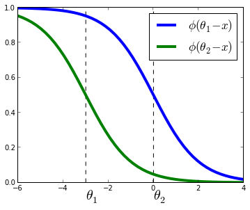
Given X∈Rn×pX∈Rn×p input data and y∈Nny∈Nn target values. For simplicity we assume yy is a non-decreasing vector, that is, y1≤y2≤...y1≤y2≤.... Just as the logistic regression models posterior probability P(y=j|Xi)P(y=j|Xi) as the logistic function, in the logistic ordinal regression we model thecummulative probability as the logistic function. That is,

P(y≤j|Xi)=ϕ(θj−wTXi)=11+exp(wTXi−θj)P(y≤j|Xi)=ϕ(θj−wTXi)=11+exp⁡(wTXi−θj)

where w,θw,θ are vectors to be estimated from the data and ϕϕ is the logistic function defined as ϕ(t)=1/(1+exp(−t))ϕ(t)=1/(1+exp⁡(−t)).

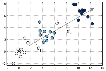
 Toy example with three classes denoted in different colors. Also shown the vector of coefficients ww and the thresholds θ0θ0 and θ1θ1

Compared to multiclass logistic regression, we have added the constrain that the hyperplanes that separate the different classes are parallel for all classes, that is, the vector ww is common across classes. To decide to which class will XiXi be predicted we make use of the vector of thresholds θθ. If there are KK different classes, θθ is a non-decreasing vector (that is, θ1≤θ2≤...≤θK−1θ1≤θ2≤...≤θK−1) of size K−1K−1. We will then assign the class jj if the prediction wTXwTX (recall that it's a linear model) lies in the interval [θj−1,θj[[θj−1,θj[. In order to keep the same definition for extremal classes, we define θ0=−∞θ0=−∞ and θK=+∞θK=+∞.

The intuition is that we are seeking a vector ww such that XwXw produces a set of values that are well separated into the different classes by the different thresholds θθ. We choose a logistic function to model the probability P(y≤j|Xi)P(y≤j|Xi) but other choices are possible. In the proportional hazards model ¹ the probability is modeled as −log(1−P(y≤j|Xi))=exp(θj−wTXi)−log⁡(1−P(y≤j|Xi))=exp⁡(θj−wTXi). Other link functions are possible, where the link function satisfies link(P(y≤j|Xi))=θj−wTXilink(P(y≤j|Xi))=θj−wTXi. Under this framework, the logistic ordinal regression model has a logistic link function and the proportional hazards model has a log-log link function.

The logistic ordinal regression model is also known as the proportional odds model, because the ratio of corresponding odds for two different samples X1X1 and X2X2 is exp(wT(X1−X2))exp⁡(wT(X1−X2)) and so does not depend on the class jj but only on the difference between the samples X1X1 and X2X2.

Optimization

Model estimation can be posed as an optimization problem. Here, we minimize the loss function for the model, defined as minus the log-likelihood:

L(w,θ)=−n∑i=1log(ϕ(θyi−wTXi)−ϕ(θyi−1−wTXi))L(w,θ)=−∑i=1nlog⁡(ϕ(θyi−wTXi)−ϕ(θyi−1−wTXi))

In this sum all terms are convex on ww, thus the loss function is convex over ww. It might be also jointly convex over ww and θθ, although I haven't checked. I use the function fmin_slsqp in scipy.optimize to optimize LLunder the constraint that θθ is a non-decreasing vector. There might be better options, I don't know. If you do know, please leave a comment!.

Using the formula log(ϕ(t))′=(1−ϕ(t))log⁡(ϕ(t))′=(1−ϕ(t)), we can compute the gradient of the loss function as

∇wL(w,θ)=n∑i=1Xi(1−ϕ(θyi−wTXi)−ϕ(θyi−1−wTXi))∇θL(w,θ)=n∑i=1eyi(1−ϕ(θyi−wTXi)−11−exp(θyi−1−θyi))+eyi−1(1−ϕ(θyi−1−wTXi)−11−exp(−(θyi−1−θyi)))∇wL(w,θ)=∑i=1nXi(1−ϕ(θyi−wTXi)−ϕ(θyi−1−wTXi))∇θL(w,θ)=∑i=1neyi(1−ϕ(θyi−wTXi)−11−exp⁡(θyi−1−θyi))+eyi−1(1−ϕ(θyi−1−wTXi)−11−exp⁡(−(θyi−1−θyi)))

where eiei is the iith canonical vector.

Code

I've implemented a Python version of this algorithm using Scipy'soptimize.fmin_slsqp function. This takes as arguments the loss function, the gradient denoted before and a function that is > 0 when the inequalities on θθ are satisfied.

Code can be found here as part of the minirank package, which is my sandbox for code related to ranking and ordinal regression. At some point I would like to submit it to scikit-learn but right now the I don't know how the code will scale to medium-scale problems, but I suspect not great. On top of that I'm not sure if there is a real demand of these models for scikit-learn and I don't want to bloat the package with unused features.

Performance

I compared the prediction accuracy of this model in the sense of mean absolute error (IPython notebook) on the boston house-prices dataset. To have an ordinal variable, I rounded the values to the closest integer, which gave me a problem of size 506 ×× 13 with 46 different target values. Although not a huge increase in accuracy, this model did give me better results on this particular dataset:

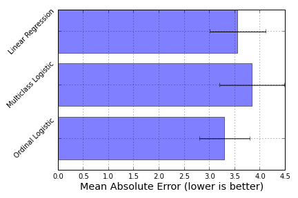
Here, ordinal logistic regression is the best-performing model, followed by a Linear Regression model and a One-versus-All Logistic regression model as implemented in scikit-learn.

python风控评分卡建模和风控常识(博客主亲自录制视频教程)

https://study.163.com/course/introduction.htm?courseId=1005214003&utm_campaign=commission&utm_source=cp-400000000398149&utm_medium=share