机器学习作业（二）逻辑回归——Matlab实现

题目太长啦！文档下载【传送门】

第1题

简述：实现逻辑回归。

第1步：加载数据文件：

data = load('ex2data1.txt');
X = data(:, [1, 2]); y = data(:, 3);
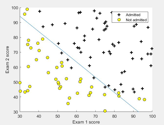
plotData(X, y);

% Put some labels
hold on;
% Labels and Legend
xlabel('Exam 1 score')
ylabel('Exam 2 score')

% Specified in plot order
legend('Admitted', 'Not admitted')
hold off;

第2步：plotData函数实现训练样本的可视化：

function plotData(X, y)
% Create New Figure
figure;
hold on;

pos = find(y==1);
neg = find(y==0);
plot(X(pos,1),X(pos,2),'k+','LineWidth',2,'MarkerSize',7);
plot(X(neg,1),X(neg,2),'ko','MarkerFaceColor','y','MarkerSize',7);

hold off;
end

第3步：计算代价函数和梯度：

%  Setup the data matrix appropriately, and add ones for the intercept term
[m, n] = size(X);

% Add intercept term to x and X_test
X = [ones(m, 1) X];

% Initialize fitting parameters
initial_theta = zeros(n + 1, 1);

% Compute and display initial cost and gradient
[cost, grad] = costFunction(initial_theta, X, y);

第4步：实现costFunction函数：

function [J, grad] = costFunction(theta, X, y)

m = length(y); % number of training examples
J = 0;
grad = zeros(size(theta));

h = sigmoid(X*theta);
J = 1/m*(-y'*log(h)-(1-y')*log(1-h));
grad = 1/m*(X'*(h-y));

end

第5步：实现sigmoid函数：

function g = sigmoid(z)
g = zeros(size(z));
g = 1./(1+exp(-z));
end

第6步：使用fminunc函数求θ和Cost：

%  Set options for fminunc
options = optimset('GradObj', 'on', 'MaxIter', 400);

%  Run fminunc to obtain the optimal theta
%  This function will return theta and the cost
[theta, cost] = ...
	fminunc(@(t)(costFunction(t, X, y)), initial_theta, options);

% Print theta to screen
fprintf('Cost at theta found by fminunc: %f\n', cost);
fprintf('theta: \n');
fprintf(' %f \n', theta);

% Plot Boundary
plotDecisionBoundary(theta, X, y);

% Put some labels
hold on;
% Labels and Legend
xlabel('Exam 1 score')
ylabel('Exam 2 score')

% Specified in plot order
legend('Admitted', 'Not admitted')
hold off;

第7步：实现plotDecisionBoundary函数：

function plotDecisionBoundary(theta, X, y)

% Plot Data
plotData(X(:,2:3), y);
hold on

if size(X, 2) <= 3
    % Only need 2 points to define a line, so choose two endpoints
    plot_x = [min(X(:,2))-2,  max(X(:,2))+2];

    % Calculate the decision boundary line
    plot_y = (-1./theta(3)).*(theta(2).*plot_x + theta(1));

    % Plot, and adjust axes for better viewing
    plot(plot_x, plot_y)

    % Legend, specific for the exercise
    legend('Admitted', 'Not admitted', 'Decision Boundary')
    axis([30, 100, 30, 100])
else
    % Here is the grid range
    u = linspace(-1, 1.5, 50);
    v = linspace(-1, 1.5, 50);

    z = zeros(length(u), length(v));
    % Evaluate z = theta*x over the grid
    for i = 1:length(u)
        for j = 1:length(v)
            z(i,j) = mapFeature(u(i), v(j))*theta;
        end
    end
    z = z'; % important to transpose z before calling contour

    % Plot z = 0
    % Notice you need to specify the range [0, 0]
    contour(u, v, z, [0, 0], 'LineWidth', 2)
end
hold off

end

运行结果：

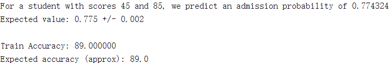
第8步：预测[45 85]成绩的学生，并计算准确率：

prob = sigmoid([1 45 85] * theta);
fprintf(['For a student with scores 45 and 85, we predict an admission ' ...
         'probability of %f\n'], prob);
fprintf('Expected value: 0.775 +/- 0.002\n\n');

% Compute accuracy on our training set
p = predict(theta, X);

fprintf('Train Accuracy: %f\n', mean(double(p == y)) * 100);
fprintf('Expected accuracy (approx): 89.0\n');
fprintf('\n');

第9步：实现predict预测函数：

function p = predict(theta, X)
m = size(X, 1); % Number of training examples
p = zeros(m, 1);
p = round(sigmoid(X*theta));
end

运行结果：

第2题

简述：通过正规化实现逻辑回归。

第1步：加载数据文件：

data = load('ex2data2.txt');
X = data(:, [1, 2]); y = data(:, 3);

plotData(X, y);

% Put some labels
hold on;

% Labels and Legend
xlabel('Microchip Test 1')
ylabel('Microchip Test 2')

% Specified in plot order
legend('y = 1', 'y = 0')
hold off;

第2步：正规化逻辑回归：

% Note that mapFeature also adds a column of ones for us, so the intercept
% term is handled
X = mapFeature(X(:,1), X(:,2));

% Initialize fitting parameters
initial_theta = zeros(size(X, 2), 1);

% Set regularization parameter lambda to 1
lambda = 1;

% Compute and display initial cost and gradient for regularized logistic
% regression
[cost, grad] = costFunctionReg(initial_theta, X, y, lambda);

fprintf('Cost at initial theta (zeros): %f\n', cost);
fprintf('Gradient at initial theta (zeros) - first five values only:\n');
fprintf(' %f \n', grad(1:5));

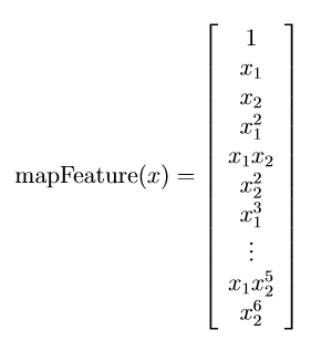
第3步：mapFeature函数实现特征设置：

function out = mapFeature(X1, X2)

degree = 6;
out = ones(size(X1(:,1)));
for i = 1:degree
    for j = 0:i
        out(:, end+1) = (X1.^(i-j)).*(X2.^j);
    end
end

end　

其设置的特征值为：

第4步：实现costFunctionReg函数：

function [J, grad] = costFunctionReg(theta, X, y, lambda)

% Initialize some useful values
m = length(y); % number of training examples

% You need to return the following variables correctly
J = 0;
grad = zeros(size(theta));

theta2 = theta(2:end,1);
h = sigmoid(X*theta);
J = 1/m*(-y'*log(h)-(1-y')*log(1-h)) + lambda/(2*m)*sum(theta2.^2);
theta(1,1) = 0;
grad = 1/m*(X'*(h-y)) + lambda/m*theta;

end

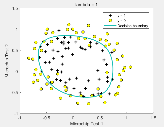
第5步：使用fminunc函数求θ和Cost，并预测准确率：

% Initialize fitting parameters
initial_theta = zeros(size(X, 2), 1);

% Set regularization parameter lambda to 1 (you should vary this)
lambda = 1;

% Set Options
options = optimset('GradObj', 'on', 'MaxIter', 400);

% Optimize
[theta, J, exit_flag] = ...
	fminunc(@(t)(costFunctionReg(t, X, y, lambda)), initial_theta, options);

% Plot Boundary
plotDecisionBoundary(theta, X, y);
hold on;
title(sprintf('lambda = %g', lambda))

% Labels and Legend
xlabel('Microchip Test 1')
ylabel('Microchip Test 2')

legend('y = 1', 'y = 0', 'Decision boundary')
hold off;

% Compute accuracy on our training set
p = predict(theta, X);

fprintf('Train Accuracy: %f\n', mean(double(p == y)) * 100);
fprintf('Expected accuracy (with lambda = 1): 83.1 (approx)\n');

运行结果：