【原】Coursera—Andrew Ng机器学习—编程作业 Programming Exercise 1 线性回归

作业说明

　　Exercise 1，Week 2，使用Octave实现线性回归模型。数据集 ex1data1.txt ，ex1data2.txt

　　单变量线性回归必须实现，实现代价函数计算Computing Cost 和梯度下降Gradient Descent。

　　多变量线性回归可选，实现特征Feature Normalization、代价函数计算Computing Cost 、梯度下降Gradient Descent 和 Normal Equations 。

文件清单

ex1.m
ex1_multi.m
ex1data1.txt - ex1.m 用到的数据组
ex1data2.txt - ex1_multi.m 用到的数据组
submit.m - 提交代码
[*] warmUpExercise.m
[*] plotData.m
[*] computeCost.m
[*] gradientDescent.m
[+] computeCostMulti.m
[+] gradientDescentMulti.m
[+] featureNormalize.m
[+] normalEqn.m

　　* 为必须要完成的
　　+ 为可

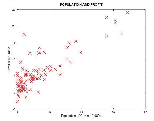
　　背景：假设我们现在是个连锁餐厅的老板，已经在很多城市开了连锁店（提供训练组），现在想再开新店，需要通过以前的数据预测新开的店的收益。

　　ex1data1.txt 提供所需要的训练组，第一列是城市人口，第二列是对应的收益。负值代表着亏损。

结论

　　当数据的特征维度比较小的时候，使用正规方程方法不需要进行特征归一化，而且结果稳定。梯度下降有可能得到局部最优解，导致结果不同。

　　注意矩阵计算的一些问题，求和前面一项需要转置。

必做题单变量线性回归

一、warmUp

　　单变量线性回归入口在ex1.m

　　warmUpExercise.m

A = eye()

二、绘制数据图

　　我实现的 plotData.m：

   plot(x,y,'rx', 'MarkerSize', );

   xlabel('Population of City in 10,000s');

   ylabel('Profit in $10,000s');

   title('POPULATION AND PROFIT');

　　 ex1.m 中的调用：

 %% ======================= Part : Plotting ======================= data = load('ex1data1.txt');

 X = data(:, ); y = data(:, );

 m = length(y); % number of training examples

  plotData(X, y);

　　运行效果如下：

三、代价函数

　　我实现的 computeCost.m：

 function J = computeCost(X, y, theta) m = length(y); % number of training examples

  J = ;

    predictions = X * theta; % predictions of hapothesis on all m examples

   sqrErrors = (predictions - y) .^ ; % squared errors .^ 指的是对数据中每个元素平方

   J =  / ( * m) * sum(sqrErrors);

 end

四、梯度下降

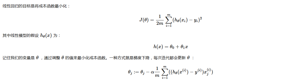
　　我实现的 gradientDescent.m

　矩阵性质：(AB)^T =B^TA^T

 function [theta, J_history, theta_history] = gradientDescent(X, y, theta, alpha, num_iters) m = length(y); % number of training examples

 J_history = zeros(num_iters, );

 theta_history = zeros(, num_iters); % 【改动】使用 ×iteration维矩阵，保存theta每次迭代的历史

 for iter = :num_iters

     % 这里为了方便理解 拆的比较细，可以组合成一步操作 theta = theta - (alpha / m) * X' * (X * theta - y)

     % prediction h(x)  m×2矩阵 * 2×1向量 = m维列向量

     predictions = X * theta;

     % error h(x)-y m维列向量

     errors = predictions - y; %

     % derivative of J()  m维行向量 * m×2矩阵 = 2维列向量

     lineLope =  X' * errors;

     % theta 2维列向量

     theta = theta - (alpha / m) * lineLope; %

          J_history(iter) = computeCost(X, y, theta);  % Save the cost J in every iteration

     theta_history(:,iter) = theta;  % 给theta_history 第iter列赋值

 end

 end

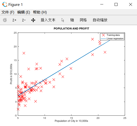
五、绘制预测曲线　　

　　ex1.m 中的调用：

 %% =================== Part : Cost and Gradient descent ===================

 % 设置 X 和 theta

 X = [ones(m, ), data(:,)]; % Add a column of ones to x

 theta = zeros(, ); % initialize fitting parameters

 % 设置迭代次数和学习速率

 iterations = ;

 alpha = 0.01;

  % compute and display initial cost      计算theta=[;]时代价

 J = computeCost(X, y, theta);

 % further testing of the cost function  计算theta=[-;]时代价

 J = computeCost(X, y, [- ; ]);

 fprintf('\nRunning Gradient Descent ...\n') % 【改动1】改为获取多个返回值，J_history保存每次迭代的代价，theta保存每次迭代的theta0和theta1

 % 原：theta = gradientDescent(X, y, theta, alpha, iterations);

 [theta,J_history,theta_history] = gradientDescent(X, y, theta, alpha, iterations);

 % Plot the linear fit 在数据图上绘制最终的拟合直线

 hold on; % keep previous plot visible

 plot(X(:,), X*theta, '-')

 legend('Training data', 'Linear regression')

 hold off % don't overlay any more plots on this figure

　　运行结果如下：

四、绘制cost和theta变化曲线

自己加的功能。在ex1.m中增加以下代码，绘制图像。展示迭代过程中 cost 和 theta 的变化曲线

 % --------------【改动2】绘制代价和theta变化曲线 start --------------

 fprintf('Size of J_history saved by gradient descent:\n');

 fprintf('%f\n', size(J_history));

 iterX = [:iterations]'; % 生成图像横坐标，迭代次数

 % 绘左侧图，展示迭代过程中代价的变化曲线

 subplot(,,);

 plot(iterX, J_history, '-','linewidth',); % 绘制代价函数曲线

 title('cost of each step'),

 xlabel('iteration'),ylabel('value of cost'),

 legend('value of cost');

 % 绘右侧图，展示迭代过程中theta的变化曲线

 theta0_history = theta_history(,:);

 theta1_history = theta_history(,:);

 subplot(,,);

 plot(iterX,theta0_history,'-','linewidth',);

 hold on;

 plot(iterX,theta1_history,'-','linewidth',,'color','r');

 title('theta of each step'),xlabel('iteration'),ylabel('value of theta'),legend('theta0','theta1');

 % --------------【改动2】绘制代价和theta变化曲线 end --------------

 % Predict values for population sizes of , and ,

 predict1 = [, 3.5] * theta;

 fprintf('For population = 35,000, we predict a profit of %f\n',...

     predict1*);

 predict2 = [, ] * theta;

 fprintf('For population = 70,000, we predict a profit of %f\n',...

     predict2*);

输出如下：

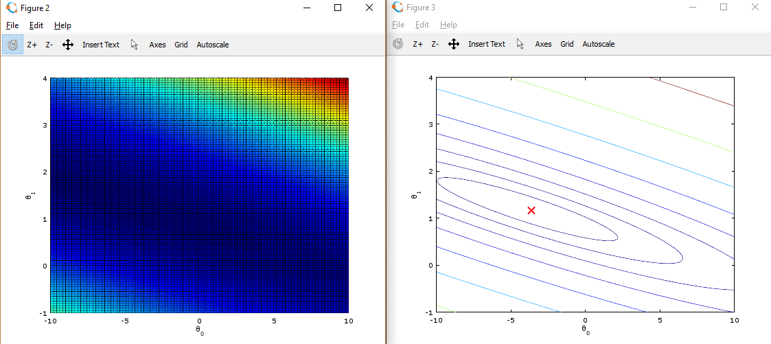
五、绘制代价函数三维曲线和等高线图

　　ex1.m 调用：

　　1、初始化 theta0 为（-10，10）均分100个点，theta1 为（-1,4）均分100个点，J_vals 为100 * 100的数组

　　这里使用了Matlab中的均分计算指令 linspace(x1,x2,N) ，用于产生x1、x2之间的N点行线性的矢量。其中x1、x2、N分别为起始值、终止值、元素个数。默认N为100。

　　2、循环计算每组（theta0，theta1），用 J_vals 保存对应的代价cost。

 %% ============= Part : Visualizing J(theta_0, theta_1) =============

 fprintf('Visualizing J(theta_0, theta_1) ...\n')

 % Grid over which we will calculate J

 theta0_vals = linspace(-, , );

 theta1_vals = linspace(-, , );

 % initialize J_vals to a matrix of 's

 J_vals = zeros(length(theta0_vals), length(theta1_vals));

 % Fill out J_vals

 for i = :length(theta0_vals)

     for j = :length(theta1_vals)

       t = [theta0_vals(i); theta1_vals(j)];

       J_vals(i,j) = computeCost(X, y, t);

     end

 end

 % Because of the way meshgrids work in the surf command, we need to

 % transpose J_vals before calling surf, or else the axes will be flipped

 J_vals = J_vals';

 % Surface plot

 figure;

 surf(theta0_vals, theta1_vals, J_vals)

 xlabel('\theta_0'); ylabel('\theta_1');

 % Contour plot

 figure;

 % Plot J_vals as  contours spaced logarithmically between 0.01 and

 contour(theta0_vals, theta1_vals, J_vals, logspace(-, , ))

 xlabel('\theta_0'); ylabel('\theta_1');

 hold on;

 plot(theta(), theta(), 'rx', 'MarkerSize', , 'LineWidth', );

　　3、将theta0作为X坐标，theta1作为Y坐标，J_vals作为Z坐标，绘制三维图形

　　4、将theta0作为X坐标，theta1作为Y坐标，绘制J_vals的等高线图

　　5、在等高线图中，标记上面求出的使代价函数最小的 theta0，theta1点的位置。在等高线中心

　　这些图像的目的是为了展示随着Θ₀ 和 Θ₁ 的改变，J值的变化。（在2D轮廓图中比3D的更直观）。最小点是Θ₀ 和 Θ₁最适点，每一步梯度下降都会更靠近这个点。

可以通过旋转看到为什么叫“轮廓图”：

选做多变量线性回归

一、特征归一化

需要用特性放缩让数据的范围缩小，使得梯度下降计算的更快：

- 计算每个特性的平均值(mean)
- 计算标准差(standard deviations)
- 特性放缩(feature scaling)

* 这里利用的是标准差(standard deviation)，也可以使用差值(max - min)。

　　featureNormalize.m 如下：

 1 function [X_norm, mu, sigma] = featureNormalize(X)

 7

 9 X_norm = X;

10 mu = zeros(1, size(X, 2)); % 1行，列数和X相同

11 sigma = zeros(1, size(X, 2));

12

13 % ====================== YOUR CODE HERE ======================

29 mu = mean(X);

30 sigma = std(X);

32 X_norm = (X_norm - mu) ./ sigma;

35

36 end

二、代价函数和梯度下降

　　因为在单变量线性回归中，使用的是向量化的计算方法，对于多变量线性回归同样适用。不需要重新写

　　 computeCostMulti.m 和 computCost.m 一样，gradientDescentMulti.m 和gradientDescent.m 一样

　　ex1_multi.m 里的调用：

 %% ================ Part : Gradient Descent ================

 alpha = 1.2;

 num_iters = ;

 % Init Theta and Run Gradient Descent

 theta = zeros(, );

 [theta,J_history] = gradientDescentMulti(X, y, theta, alpha, num_iters);

 % Plot the convergence graph

 figure;

 plot(:numel(J_history), J_history, '-b', 'LineWidth', );

 xlabel('Number of iterations');

 ylabel('Cost J');

 % Estimate the price of a  sq-ft,  br house

 % 这里要注意，需要把输入的值进行 normalize，然后才能代入预测方程中

 predict_x = [,];

 predict_x = (predict_x - mu) ./ sigma;

 price = [, predict_x] * theta;

三、正规方程

　　公式：

　　normalEqn.m 实现：

 function [theta] = normalEqn(X, y)

 theta = zeros(size(X, ), );

 theta = pinv(X' * X) * X' * y

 end

　　ex1_multi 里的调用：

 %% ================ Part : Normal Equations ================

 %  predict the price of a  sq-ft,  br house. data = csvread('ex1data2.txt');   % 重新加载数据

 X = data(:, :);

 y = data(:, );

 m = length(y);

 % Add intercept term to X

 X = [ones(m, ) X];

 % Calculate the parameters from the normal equation

 theta = normalEqn(X, y);      % 使用正规方程进行计算

28 % ====================== YOUR CODE HERE ======================

 price = [, , ] * theta; % 预测结果   % ============================================================

四、测试

　　运行结果：

 Loading data ...

 First  examples from the dataset:

  x = [ ], y =

  x = [ ], y =

  x = [ ], y =

  x = [ ], y =

  x = [ ], y =

  x = [ ], y =

  x = [ ], y =

  x = [ ], y =

  x = [ ], y =

  x = [ ], y =

 Program paused. Press enter to continue.

 Normalizing Features ...

    1.00000000   0.13000987  -0.22367519

    1.00000000  -0.50418984  -0.22367519

    1.00000000   0.50247636  -0.22367519

    1.00000000  -0.73572306  -1.53776691

    1.00000000   1.25747602   1.09041654

    1.00000000  -0.01973173   1.09041654

    1.00000000  -0.58723980  -0.22367519

    1.00000000  -0.72188140  -0.22367519

    1.00000000  -0.78102304  -0.22367519

    1.00000000  -0.63757311  -0.22367519

    1.00000000  -0.07635670   1.09041654

    1.00000000  -0.00085674  -0.22367519

    1.00000000  -0.13927334  -0.22367519

    1.00000000   3.11729182   2.40450826

    1.00000000  -0.92195631  -0.22367519

    1.00000000   0.37664309   1.09041654

 Running gradient descent ...

 Theta computed from gradient descent:

  334302.063993

  100087.116006

  3673.548451

　　（1）当 α = 0.05，预测一个1650 sq-ft, 3 br house 的房屋的售价。梯度下降和正规方程的预测值不同：

68 Predicted price of a 1650 sq-ft, 3 br house (using gradient descent):

69  $289314.620338

81

82 Predicted price of a 1650 sq-ft, 3 br house (using normal equations):

83  $293081.464335

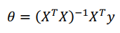
　（2）当 α = 0.15，cost 曲线如下。两个方法预测值都是 $293081.464335：

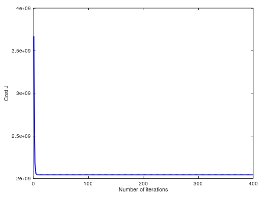
　（3）当 α = 1，cost 曲线如下。两个方法预测值都是 $293081.464335：

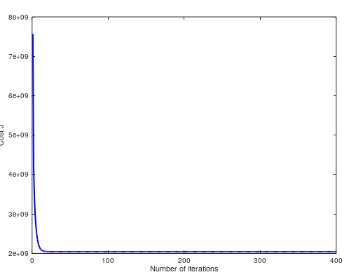
　（4）当 α = 1.2，cost 曲线如下。两个方法预测值都是 $293081.464335：

　（5）当 α = 1.3，cost 曲线如下。两个方法预测值不同 $293157.248289 ，$293081.464335：　

　　完整代码：https://github.com/madoubao/coursera_machine_learning/tree/master/homework/machine-learning-ex1/ex1