机器学习入门-随机森林温度预测的案例 1.datetime.datetime.datetime(将字符串转为为日期格式) 2.pd.get_dummies(将文本标签转换为one-hot编码) 3.rf.feature_importances_(研究样本特征的重要性) 4.fig.autofmt_xdate(rotation=60) 对标签进行翻转

在这个案例中：

1. datetime.datetime.strptime(data, '%Y-%m-%d') # 由字符串格式转换为日期格式

2. pd.get_dummies(features)  # 将数据中的文字标签转换为one-hot编码形式，增加了特征的列数

3. rf.feature_importances 探究了随机森林样本特征的重要性，对其进行排序后条形图

4.fig.autofmt_xdate(rotation=60)  # 对图中的X轴标签进行60的翻转

代码：

第一步：数据读取，通过.describe() 查看数据是否存在缺失值的情况

第二步：对年月日特征进行字符串串接，使用datetime.datetime.strptime(), 获得日期格式作为X轴的标签

第三步：对里面的几个温度特征做条形图，fig.autofmt_xdate(rotation=60)设置日期标签的旋转角度，plt.style.use('fivethirtyeight') 设置画风

第四步：使用pd.get_dummies(features) 将特征中文字类的标签转换为one-hot编码形式，增加了特征的维度

第五步：提取数据的特征和样本标签，转换为np.array格式

第六步：使用train_test_split 将特征和标签分为训练集和测试集

第七步：构建随机森林模型进行模型的训练和预测

第八步：进行随机森林的可视化

第九步：使用rf.feature_importances_计算出各个特征的重要性，进行排序，然后做条形图

第十步：根据第九步求得的特征重要性的排序结果，我们选用前两个特征建立模型和预测

第十一步：对模型的预测结果画直线图plot和散点图scatter，对于plot我们需要根据时间进行排序

import numpy as np
import pandas as pd
import matplotlib.pyplot as plt
import datetime

# 第一步提取数据
features = pd.read_csv('data/temps.csv')
print(features.shape)
print(features.columns)
# 使用feature.describe()   # 观察数据是否存在缺失值
print(features.describe())

# 第二步：我们将year,month,day特征组合成一个dates特征，作为画图的标签值比如2016-02-01

years = features['year']
months = features['month']
days = features['day']

# datetime.datetime.strptime() 将字符串转换为日期类型
dates = [str(int(year)) + '-' + str(int(month)) + '-' + str(int(day)) for year, month, day in zip(years, months, days)]
dates = [datetime.datetime.strptime(date, '%Y-%m-%d') for date in dates]
print(dates[0:5])

# 第三步进行画图操作
# 设置画图风格
plt.style.use('fivethirtyeight')

# 使用plt.subplots画出多副图
fig, ((ax1, ax2), (ax3, ax4)) = plt.subplots(ncols=2, nrows=2, figsize=(12, 12))
# 使得标签进行角度翻转
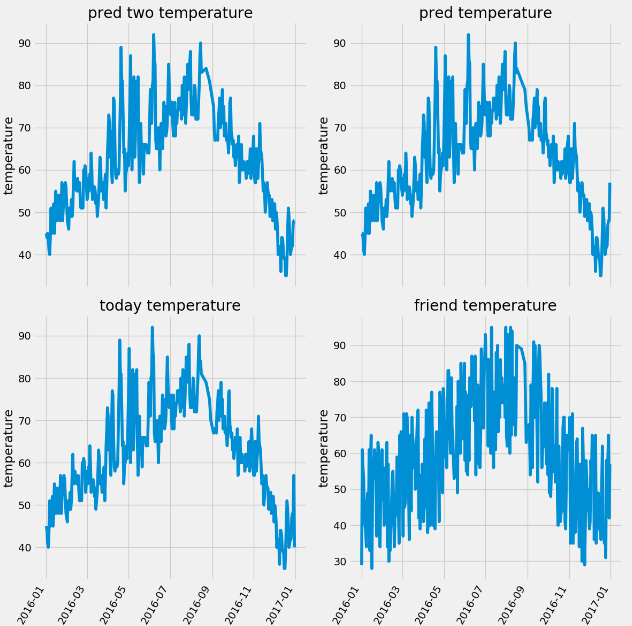
fig.autofmt_xdate(rotation=60)

ax1.plot(dates, features['temp_2'], linewidth=4)
ax1.set_xlabel(''), ax1.set_ylabel('temperature'), ax1.set_title('pred two temperature')

ax2.plot(dates, features['temp_1'], linewidth=4)
ax2.set_xlabel(''), ax1.set_ylabel('temperature'), ax1.set_title('pred temperature')

ax3.plot(dates, features['actual'], linewidth=4)
ax3.set_xlabel(''), ax1.set_ylabel('temperature'), ax1.set_title('today temperature')

ax4.plot(dates, features['friend'], linewidth=4)
ax4.set_xlabel(''), ax1.set_ylabel('temperature'), ax1.set_title('friend temperature')

plt.show()

# 第四步：pd.get_dummies() 来对特征中不是数字的特征进行one-hot编码
features = pd.get_dummies(features)

# 第五步：把数据分为特征和标签

y = np.array(features['actual'])
X = features.drop('actual', axis=1)
feature_names = list(X.columns)
X = np.array(X)

# 第六步： 使用train_test_split 对数据进行拆分
from sklearn.model_selection import train_test_split

train_X, test_X, train_y, test_y = train_test_split(X, y, test_size=0.25, random_state=42)

# 第七步：建立随机森林的模型进行预测
from sklearn.ensemble import RandomForestRegressor

rf = RandomForestRegressor(n_estimators=1000)
rf.fit(train_X, train_y)
pred_y = rf.predict(test_X)

# MSE指标通过真实值-预测值的绝对值求平均值
MSE = round(abs(pred_y - test_y).mean(), 2)

# MAPE指标通过 1 - abs(误差)/真实值来表示
error = abs(pred_y - test_y)

MAPE = round(np.mean((1 - error / test_y) * 100), 2)

print(MSE, MAPE)

# 第八步进行随机森林的可视化展示

# from sklearn.tree import export_graphviz
# import pydot #pip install pydot
#
# # Pull out one tree from the forest
# tree = model.estimators_[5]
#
# # Export the image to a dot file
# export_graphviz(tree, out_file = 'tree.dot', feature_names = feature_names, rounded = True, precision = 1)
#
# # Use dot file to create a graph
# (graph, ) = pydot.graph_from_dot_file('tree.dot')
# graph.write_png('tree.png');
# print('The depth of this tree is:', tree.tree_.max_depth)
#
# # 限制树的深度重新画图
# rf_small = RandomForestRegressor(n_estimators=10, max_depth = 3, random_state=42)
# rf_small.fit(train_x,train_y)
#
# # Extract the small tree
# tree_small = rf_small.estimators_[5]
#
# # Save the tree as a png image
# export_graphviz(tree_small, out_file = 'small_tree.dot', feature_names = feature_names, rounded = True, precision = 1)
#
# (graph, ) = pydot.graph_from_dot_file('small_tree.dot')
#
# graph.write_png('small_tree.png')

#第九步：探讨随机森林特征的重要性
features_importances = rf.feature_importances_
features_importance_pairs = [(feature_name, features_importance) for feature_name, features_importance in
                             zip(feature_names, features_importances)]
# 对里面的特征进行排序操作
features_importance_pairs = sorted(features_importance_pairs, key=lambda x: x[1], reverse=True)
features_importance_name = [name[0] for name in features_importance_pairs]
features_importance_val = [name[1] for name in features_importance_pairs]

figure = plt.figure()
plt.bar(range(len(features_importance_name)), features_importance_val, orientation='vertical')
plt.xticks(range(len(features_importance_name)), features_importance_name, rotation='vertical')
plt.show()

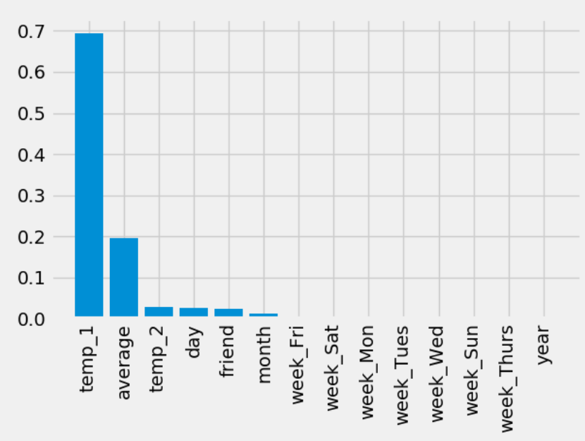
# 第十步：通过上述的作图，我们可以发现前两个特征很重要，因此我们只选用前两个特征作为训练数据

X = features.drop('actual', axis=1)
y = np.array(features['actual'])

train_x, test_x, train_y, test_y = train_test_split(X, y, test_size=0.25, random_state=42)

train_x_two = train_x[['temp_1', 'average']].values
test_x_two = test_x[['temp_1', 'average']].values

rf = RandomForestRegressor(n_estimators=1000)
rf.fit(train_x_two, train_y)
pred_y = rf.predict(test_x_two)

# MSE指标通过真实值-预测值的绝对值求平均值
MSE = round(abs(pred_y - test_y).mean(), 2)

# MAPE指标通过 1 - abs(误差)/真实值来表示
error = abs(pred_y - test_y)

MAPE = round(np.mean((1 - error / test_y) * 100), 2)
print(MSE, MAPE)

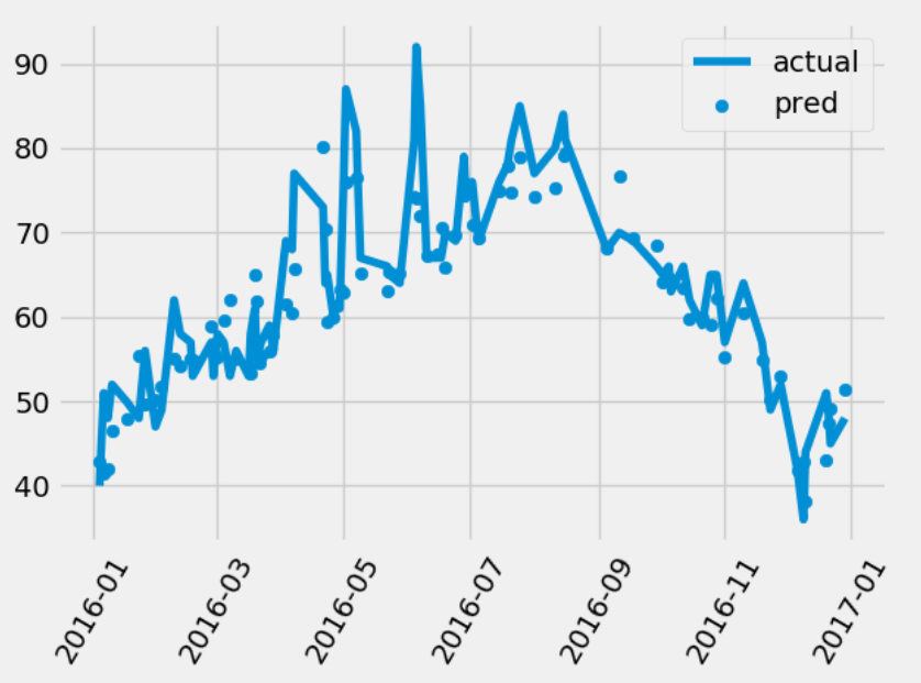
# 我们发现只使用两个特征也是具有差不多的结果，因此我们可以通过减少特征来增加反应的时间

fig = plt.figure()

years = test_x['year']
months = test_x['month']
days = test_x['day']

dates = [str(int(year)) + '-' + str(int(month)) + '-' + str(int(day)) for year, month, day in zip(years, months, days)]
dates = [datetime.datetime.strptime(date, '%Y-%m-%d') for date in dates]
print(dates[0:5])

# 对真实的数据进行排序，因为需要画plot图
dates_test_paris = [(date, test_) for date, test_ in zip(dates, test_y)]
dates_test_paris = sorted(dates_test_paris, key=lambda x: x[0], reverse=True)
dates_test_data = [x[0] for x in dates_test_paris]
dates_test_val = [x[1] for x in dates_test_paris]

plt.plot(dates_test_data, dates_test_val, label='actual')
plt.scatter(dates, pred_y, label='pred')
plt.xticks(rotation='')
plt.legend()
plt.show()