《DSP using MATLAB》示例Example 8.26

代码：

%% ------------------------------------------------------------------------
%%            Output Info about this m-file
fprintf('\n***********************************************************\n');
fprintf('        <DSP using MATLAB> Exameple 8.26 \n\n');

time_stamp = datestr(now, 31);
[wkd1, wkd2] = weekday(today, 'long');
fprintf('      Now is %20s, and it is %8s  \n\n', time_stamp, wkd2);
%% ------------------------------------------------------------------------

% Digital Lowpass Filter Specifications:
wplp = 0.2*pi;                 % digital passband freq in rad
wslp = 0.3*pi;                 % digital stopband freq in rad
  Rp = 1;                      % passband ripple in dB
  As = 15;                     % stopband attenuation in dB

% Analog prototype specifications: Inverse Mapping for frequencies
T = 1;  Fs = 1/T;                  % set T = 1
OmegaP = (2/T)*tan(wplp/2);        % Prewarp(Cutoff) prototype passband freq
OmegaS = (2/T)*tan(wslp/2);        % Prewarp(cutoff) prototype stopband freq

% Analog Chebyshev-1 Prototype Filter Calculations:
[cs, ds] = afd_chb1(OmegaP, OmegaS, Rp, As);

% Bilinear transformation to obtain digital lowpass:
[blp, alp] = bilinear(cs, ds, Fs);

% Digital Highpass Filter Design:
wphp = 0.6*pi;                        % Digital HP cutoff freq, passband edge freq

% LP-to-HP frequency-band transfromation:
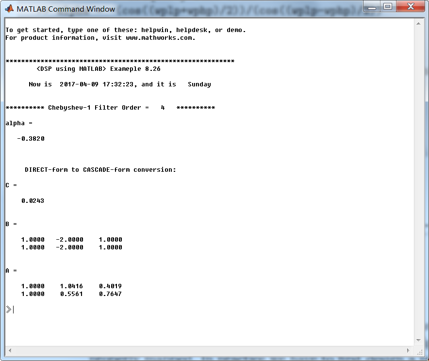
alpha = -(cos((wplp+wphp)/2))/(cos((wplp-wphp)/2))
Nz = -[alpha, 1]; Dz = [1, alpha];

[bhp, ahp] = zmapping(blp, alp, Nz, Dz); [C, B, A] = dir2cas(bhp, ahp)

% Calculation of Frequency Response:
[dblp, maglp, phalp, grdlp, wwlp] = freqz_m(blp, alp);
[dbhp, maghp, phahp, grdhp, wwhp] = freqz_m(bhp, ahp);

%% -----------------------------------------------------------------
%%                             Plot
%% -----------------------------------------------------------------  

figure('NumberTitle', 'off', 'Name', 'Exameple 8.26a')
set(gcf,'Color','white');
M = 1;                          % Omega max

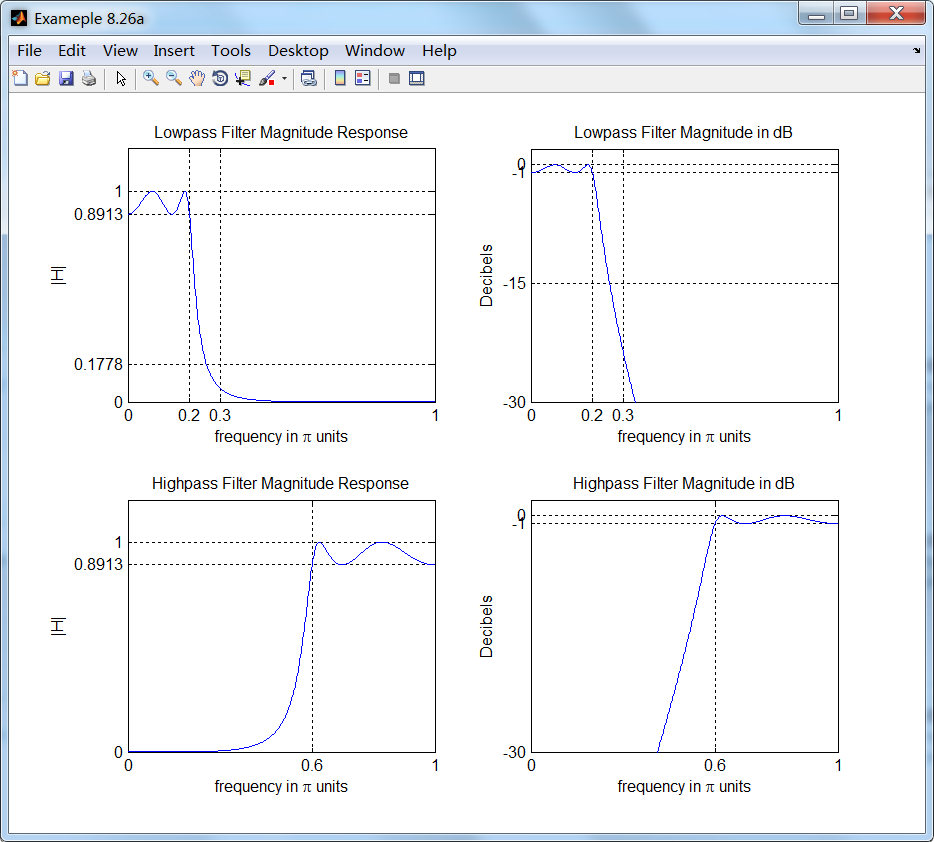
subplot(2,2,1); plot(wwlp/pi, maglp); axis([0, M, 0, 1.2]); grid on;
xlabel(' frequency in \pi units'); ylabel('|H|'); title('Lowpass Filter Magnitude Response');
set(gca, 'XTickMode', 'manual', 'XTick', [0, 0.2, 0.3, M]);
set(gca, 'YTickMode', 'manual', 'YTick', [0, 0.1778, 0.8913, 1]);

subplot(2,2,2); plot(wwlp/pi, dblp); axis([0, M, -30, 2]); grid on;
xlabel(' frequency in \pi units'); ylabel('Decibels'); title('Lowpass Filter Magnitude in dB');
set(gca, 'XTickMode', 'manual', 'XTick', [0, 0.2, 0.3, M]);
set(gca, 'YTickMode', 'manual', 'YTick', [-30, -15, -1, 0]);

subplot(2,2,3); plot(wwhp/pi, maghp); axis([0, M, 0, 1.2]); grid on;
xlabel(' frequency in \pi units'); ylabel('|H|'); title('Highpass Filter Magnitude Response');
set(gca, 'XTickMode', 'manual', 'XTick', [0, 0.6, M]);
set(gca, 'YTickMode', 'manual', 'YTick', [0, 0.8913, 1]);

subplot(2,2,4); plot(wwhp/pi, dbhp); axis([0, M, -30, 2]); grid on;
xlabel(' frequency in \pi units'); ylabel('Decibels'); title('Highpass Filter Magnitude in dB');
set(gca, 'XTickMode', 'manual', 'XTick', [0, 0.6, M]);
set(gca, 'YTickMode', 'manual', 'YTick', [-30, -1, 0]);

figure('NumberTitle', 'off', 'Name', 'Exameple 8.26b')
set(gcf,'Color','white'); 

subplot(2,2,1); plot(wwlp/pi, phalp/pi); axis([0, M, -1.1, 1.1]); grid on;
xlabel('frequency in \pi nuits'); ylabel('radians in \pi units'); title('Lowpass Filter Phase Response');
set(gca, 'XTickMode', 'manual', 'XTick', [0, 0.2, 0.3, M]);
set(gca, 'YTickMode', 'manual', 'YTick', [-1:1:1]);

subplot(2,2,2); plot(wwlp/pi, grdlp); axis([0, M, 0, 15]); grid on;
xlabel('frequency in \pi units'); ylabel('Samples'); title('Lowpass Filter Group Delay');
set(gca, 'XTickMode', 'manual', 'XTick', [0, 0.2, 0.3, M]);
set(gca, 'YTickMode', 'manual', 'YTick', [0:5:15]);

subplot(2,2,3); plot(wwhp/pi, phahp/pi); axis([0, M, -1.1, 1.1]); grid on;
xlabel('frequency in \pi nuits'); ylabel('radians in \pi units'); title('Highpass Filter Phase Response');
set(gca, 'XTickMode', 'manual', 'XTick', [0, 0.6, M]);
set(gca, 'YTickMode', 'manual', 'YTick', [-1:1:1]);

subplot(2,2,4); plot(wwhp/pi, grdhp); axis([0, M, 0, 15]); grid on;
xlabel('frequency in \pi units'); ylabel('Samples'); title('Highpass Filter Group Delay');
set(gca, 'XTickMode', 'manual', 'XTick', [0, 0.6, M]);
set(gca, 'YTickMode', 'manual', 'YTick', [0:5:15]);

　　运行结果：