(原)Non-local Neural Networks
转载请注明出处:
https://www.cnblogs.com/darkknightzh/p/12592351.html
论文:
https://arxiv.org/abs/1711.07971
第三方pytorch代码:
https://github.com/AlexHex7/Non-local_pytorch
1. non local操作
该论文定义了通用了non local操作:
${{\mathbf{y}}_{i}}=\frac{1}{C(\mathbf{x})}\sum\limits_{\forall j}{f({{\mathbf{x}}_{i}},{{\mathbf{x}}_{j}})g({{\mathbf{x}}_{j}})}$
其中i为需要计算响应的输出位置的索引,j为所有的位置。x为输入信号(图像,序列,视频等,通常为这些信号的特征),y为个x相同尺寸的输出信号。f为pairwise的函数,f计算当前i和所有j之间的关系,并得到一个标量。一元函数g计算输入信号在位置j的表征。(这段翻译起来怪怪的)。C(x)为归一化系数,用于归一化f和g的结果。
2. non local和其他操作的区别
① non local考虑到了所有的位置j。卷积操作仅考虑了当前位置的一个邻域(如核为3的一维卷积仅考虑了i-1<=j<=i+1);循环操作通常只考虑当前和上一个时间,j=i或j=i-1.
② non local根据不同位置的关系计算响应,fc使用学习到的权重。换言之,fc中,${{\mathbf{x}}_{i}}$和${{\mathbf{x}}_{j}}$之间不是函数关系,而non local中则是函数关系。
③ non local支持输入不同尺寸,并且保持输出和输入相同的尺寸;fc则需要输入和输出均为固定的尺寸,并且丢失了位置关系。
④ non local可以用在网络的早期部分,fc通常用在网络最后。
3. f和g的形式
3.1 g的形式
为简单起见,只考虑g为线性形式,$g({{\mathbf{x}}_{j}})\text{=}{{W}_{g}}{{\mathbf{x}}_{j}}$,${{W}_{g}}$为需要学习的权重向量,在空域可以使用1*1conv实现,在空间时间域(如时间序列的图像)可以通过1*1*1的卷积实现。
3.2 f为gaussian
$f({{\mathbf{x}}_{i}},{{\mathbf{x}}_{j}})\text{=}{{e}^{\mathbf{x}_{i}^{T}{{\mathbf{x}}_{j}}}}$
其中$\mathbf{x}_{i}^{T}{{\mathbf{x}}_{j}}$为点乘,因为点乘在深度学习平台中更易实现(欧式距离也可以)。此时归一化系数$C(\mathbf{x})=\sum\nolimits_{\forall j}{f({{\mathbf{x}}_{i}},{{\mathbf{x}}_{j}})}$
3.3 f为embedded Gaussian
$f({{\mathbf{x}}_{i}},{{\mathbf{x}}_{j}})\text{=}{{e}^{\theta {{({{\mathbf{x}}_{i}})}^{T}}\phi ({{\mathbf{x}}_{j}})}}$
其中$\theta ({{\mathbf{x}}_{i}})\text{=}{{W}_{\theta }}{{\mathbf{x}}_{i}}$,$\phi ({{\mathbf{x}}_{j}})\text{=}{{W}_{\phi }}{{\mathbf{x}}_{j}}$,此时$C(\mathbf{x})=\sum\nolimits_{\forall j}{f({{\mathbf{x}}_{i}},{{\mathbf{x}}_{j}})}$
self attention模块和non local的关系:可以认为self attention为embedded Gaussian的特殊形式,如给定i,$\frac{1}{C(\mathbf{x})}f({{\mathbf{x}}_{i}},{{\mathbf{x}}_{j}})$沿着j维度变成了计算softmax。此时$\mathbf{y}=softmax({{\mathbf{x}}^{T}}W_{\theta }^{T}{{W}_{\phi }}\mathbf{x})g(\mathbf{x})$,即为self attention的形式。
3.4 点乘
f可以定义为点乘的相似度(此处使用embedded的形式):
$f({{\mathbf{x}}_{i}},{{\mathbf{x}}_{j}})\text{=}\theta {{({{\mathbf{x}}_{i}})}^{T}}\phi ({{\mathbf{x}}_{j}})$
此时,归一化系数$C(\mathbf{x})=N$,N为x中所有位置的数量,而不是f的sum,这样可以简化梯度的计算。
点乘和embedded Gaussian的区别是是否使用了作为激活函数的softmax。
3.5 Concatenation
$f({{\mathbf{x}}_{i}},{{\mathbf{x}}_{j}})\text{=ReLU(w}_{f}^{T}[\theta ({{\mathbf{x}}_{i}}),\phi ({{\mathbf{x}}_{j}})]\text{)}$
其中$[\cdot \cdot ]$代表concatenation,即拼接。${{w}_{f}}$为权重向量,用于将拼接后的向量映射到一个标量。$C(\mathbf{x})=N$
4. Non local block
将之前公式的non local操作扩展成non local block,可以嵌入到目前的网络结构中,如下:
${{\mathbf{z}}_{i}}={{W}_{z}}{{\mathbf{y}}_{i}}+{{\mathbf{x}}_{i}}$
其中${{\mathbf{y}}_{i}}=\frac{1}{C(\mathbf{x})}\sum\limits_{\forall j}{f({{\mathbf{x}}_{i}},{{\mathbf{x}}_{j}})g({{\mathbf{x}}_{j}})}$,$+{{\mathbf{x}}_{i}}$代表残差连接。残差连接方便将non local block嵌入到之前与训练的模型中,避免打乱其初始行为(如将${{W}_{z}}$初始化为0)。
non local block如下图所示。3.2,3.3,3.4中的pairwise计算对应于下图中的矩阵乘法。在网络后面的特征图上,pairwise计算量比较小。
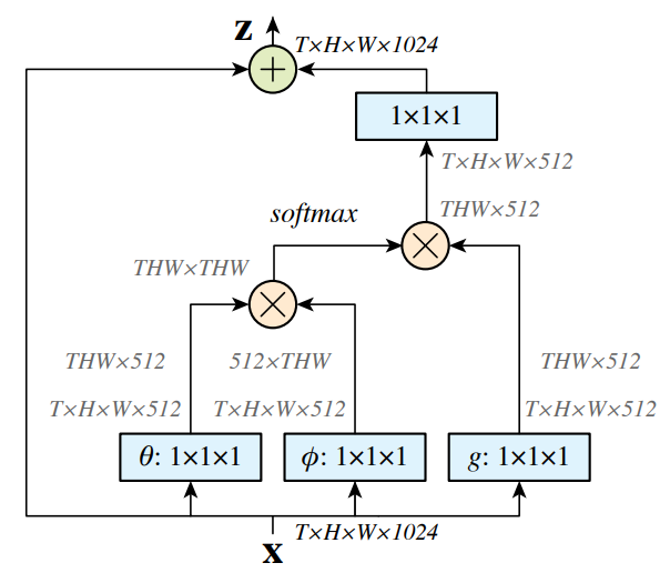
说明:
1. 若为图像,则使用1*1conv,且图中无T;若为视频,则使用1*1*1conv,且图中有T。
2. 图中softmax指对该矩阵每行计算softmax。
5. 降低计算量
5.1 降低x的通道数量
将${{W}_{g}}$,${{W}_{\theta }}$,${{W}_{\phi }}$降低为x的通道数量的一半,可以降低计算量。
5.2 对x下采样。
对x下采样,可以进一步降低计算量。
此时,1中的共识修改为${{\mathbf{y}}_{i}}=\frac{1}{C(\mathbf{\hat{x}})}\sum\limits_{\forall j}{f({{\mathbf{x}}_{i}},{{{\mathbf{\hat{x}}}}_{j}})g({{{\mathbf{\hat{x}}}}_{j}})}$,其中$\mathbf{\hat{x}}$为对x进行下采样后的输入(如pooling)。这种方式可以降低pariwsie计算到原来的1/4,一方面不影响non local的行为,另一方面,使得计算更加稀疏。可以通过在上图中$\phi $和$g$后面加一个max pooling来实现。
6. 代码:
6.1 embedded_gaussian
 class _NonLocalBlockND(nn.Module):

     def __init__(self, in_channels, inter_channels=None, dimension=3, sub_sample=True, bn_layer=True):

         """

         :param in_channels:

         :param inter_channels:

         :param dimension:

         :param sub_sample:

         :param bn_layer:

         """

         super(_NonLocalBlockND, self).__init__()

         assert dimension in [1, 2, 3]

         self.dimension = dimension

         self.sub_sample = sub_sample

         self.in_channels = in_channels

         self.inter_channels = inter_channels

         if self.inter_channels is None:

             self.inter_channels = in_channels // 2

             if self.inter_channels == 0:

                 self.inter_channels = 1

         if dimension == 3:

             conv_nd = nn.Conv3d

             max_pool_layer = nn.MaxPool3d(kernel_size=(1, 2, 2))

             bn = nn.BatchNorm3d

         elif dimension == 2:

             conv_nd = nn.Conv2d

             max_pool_layer = nn.MaxPool2d(kernel_size=(2, 2))

             bn = nn.BatchNorm2d

         else:

             conv_nd = nn.Conv1d

             max_pool_layer = nn.MaxPool1d(kernel_size=(2))

             bn = nn.BatchNorm1d

         self.g = conv_nd(in_channels=self.in_channels, out_channels=self.inter_channels,

                          kernel_size=1, stride=1, padding=0)    # g函数,1*1conv,用于降维

         if bn_layer:

             self.W = nn.Sequential(    # 1*1conv,用于图2中变换到原始维度

                 conv_nd(in_channels=self.inter_channels, out_channels=self.in_channels,

                         kernel_size=1, stride=1, padding=0),

                 bn(self.in_channels)

             )

             nn.init.constant_(self.W[1].weight, 0)

             nn.init.constant_(self.W[1].bias, 0)

         else:

             self.W = conv_nd(in_channels=self.inter_channels, out_channels=self.in_channels,

                              kernel_size=1, stride=1, padding=0)   # 1*1conv,用于图2中变换到原始维度

             nn.init.constant_(self.W.weight, 0)

             nn.init.constant_(self.W.bias, 0)

         self.theta = conv_nd(in_channels=self.in_channels, out_channels=self.inter_channels,

                              kernel_size=1, stride=1, padding=0)   # θ函数,1*1conv,用于降维

         self.phi = conv_nd(in_channels=self.in_channels, out_channels=self.inter_channels,

                            kernel_size=1, stride=1, padding=0)    # φ函数,1*1conv,用于降维

         if sub_sample:

             self.g = nn.Sequential(self.g, max_pool_layer)

             self.phi = nn.Sequential(self.phi, max_pool_layer)

     def forward(self, x, return_nl_map=False):

         """

         :param x: (b, c, t, h, w)

         :param return_nl_map: if True return z, nl_map, else only return z.

         :return:

         """

         # 令x维度B*C*(K):一维时,x为B*C*(K1);二维时,x为B*C*(K1*K2);三维时,x为B*C*(K1*K2*K3)

         batch_size = x.size(0)   # batchsize

         g_x = self.g(x).view(batch_size, self.inter_channels, -1)   # 通过g函数,并reshape,得到B*inter_channels*(K)矩阵

         g_x = g_x.permute(0, 2, 1)   # 得到B*(K)*inter_channels矩阵,和图2中一致

         theta_x = self.theta(x).view(batch_size, self.inter_channels, -1)   # 通过θ函数,并reshape,得到B*inter_channels*(K)矩阵

         theta_x = theta_x.permute(0, 2, 1)   # 得到B*(K)*inter_channels矩阵,和图2中一致

         phi_x = self.phi(x).view(batch_size, self.inter_channels, -1)   # 通过φ函数,并reshape,得到B*inter_channels*(K)矩阵

         f = torch.matmul(theta_x, phi_x)    # 得到B*(K)*(K)矩阵,和图2中一致

         f_div_C = F.softmax(f, dim=-1)      # 通过softmax,对最后一维归一化,得到归一化的特征,即概率,B*(K)*(K)

         y = torch.matmul(f_div_C, g_x)      # 得到B*(K)*inter_channels矩阵,和图2中一致

         y = y.permute(0, 2, 1).contiguous() # 得到B*inter_channels*(K)矩阵,和图2中一致

         y = y.view(batch_size, self.inter_channels, *x.size()[2:])  # 得到B*inter_channels*(K1或K1*K2或K1*K2*K3)矩阵,和图2中一致

         W_y = self.W(y)  # 得到B*C*(K)矩阵,和图2中一致

         z = W_y + x   # 特征图和non local的图相加,得到新的特征图,B*C*(K)

         if return_nl_map:

             return z, f_div_C   # 返回结果及归一化的特征

         return z

 class NONLocalBlock1D(_NonLocalBlockND):

     def __init__(self, in_channels, inter_channels=None, sub_sample=True, bn_layer=True):

         super(NONLocalBlock1D, self).__init__(in_channels,

                                               inter_channels=inter_channels,

                                               dimension=1, sub_sample=sub_sample,

                                               bn_layer=bn_layer)

 class NONLocalBlock2D(_NonLocalBlockND):

     def __init__(self, in_channels, inter_channels=None, sub_sample=True, bn_layer=True):

         super(NONLocalBlock2D, self).__init__(in_channels,

                                               inter_channels=inter_channels,

                                               dimension=2, sub_sample=sub_sample,

                                               bn_layer=bn_layer,)

 class NONLocalBlock3D(_NonLocalBlockND):

     def __init__(self, in_channels, inter_channels=None, sub_sample=True, bn_layer=True):

         super(NONLocalBlock3D, self).__init__(in_channels,

                                               inter_channels=inter_channels,

                                               dimension=3, sub_sample=sub_sample,

                                               bn_layer=bn_layer,)

 if __name__ == '__main__':

     import torch

     for (sub_sample_, bn_layer_) in [(True, True), (False, False), (True, False), (False, True)]:

         img = torch.zeros(2, 3, 20)

         net = NONLocalBlock1D(3, sub_sample=sub_sample_, bn_layer=bn_layer_)

         out = net(img)

         print(out.size())

         img = torch.zeros(2, 3, 20, 20)

         net = NONLocalBlock2D(3, sub_sample=sub_sample_, bn_layer=bn_layer_, store_last_batch_nl_map=True)

         out = net(img)

         print(out.size())

         img = torch.randn(2, 3, 8, 20, 20)

         net = NONLocalBlock3D(3, sub_sample=sub_sample_, bn_layer=bn_layer_, store_last_batch_nl_map=True)

         out = net(img)

         print(out.size())
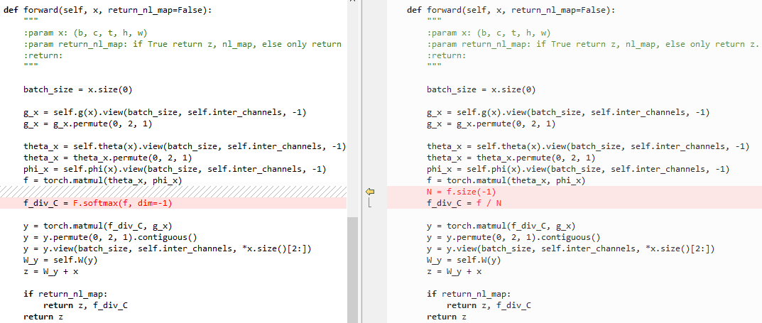
6.2 embedded Gaussian和点乘的区别
点乘代码:
 class _NonLocalBlockND(nn.Module):

     def __init__(self, in_channels, inter_channels=None, dimension=3, sub_sample=True, bn_layer=True):

         super(_NonLocalBlockND, self).__init__()

         assert dimension in [1, 2, 3]

         self.dimension = dimension

         self.sub_sample = sub_sample

         self.in_channels = in_channels

         self.inter_channels = inter_channels

         if self.inter_channels is None:

             self.inter_channels = in_channels // 2

             if self.inter_channels == 0:

                 self.inter_channels = 1

         if dimension == 3:

             conv_nd = nn.Conv3d

             max_pool_layer = nn.MaxPool3d(kernel_size=(1, 2, 2))

             bn = nn.BatchNorm3d

         elif dimension == 2:

             conv_nd = nn.Conv2d

             max_pool_layer = nn.MaxPool2d(kernel_size=(2, 2))

             bn = nn.BatchNorm2d

         else:

             conv_nd = nn.Conv1d

             max_pool_layer = nn.MaxPool1d(kernel_size=(2))

             bn = nn.BatchNorm1d

         self.g = conv_nd(in_channels=self.in_channels, out_channels=self.inter_channels,

                          kernel_size=1, stride=1, padding=0)

         if bn_layer:

             self.W = nn.Sequential(

                 conv_nd(in_channels=self.inter_channels, out_channels=self.in_channels,

                         kernel_size=1, stride=1, padding=0),

                 bn(self.in_channels)

             )

             nn.init.constant_(self.W[1].weight, 0)

             nn.init.constant_(self.W[1].bias, 0)

         else:

             self.W = conv_nd(in_channels=self.inter_channels, out_channels=self.in_channels,

                              kernel_size=1, stride=1, padding=0)

             nn.init.constant_(self.W.weight, 0)

             nn.init.constant_(self.W.bias, 0)

         self.theta = conv_nd(in_channels=self.in_channels, out_channels=self.inter_channels,

                              kernel_size=1, stride=1, padding=0)

         self.phi = conv_nd(in_channels=self.in_channels, out_channels=self.inter_channels,

                            kernel_size=1, stride=1, padding=0)

         if sub_sample:

             self.g = nn.Sequential(self.g, max_pool_layer)

             self.phi = nn.Sequential(self.phi, max_pool_layer)

     def forward(self, x, return_nl_map=False):

         """

         :param x: (b, c, t, h, w)

         :param return_nl_map: if True return z, nl_map, else only return z.

         :return:

         """

         # 令x维度B*C*(K):一维时,x为B*C*(K1);二维时,x为B*C*(K1*K2);三维时,x为B*C*(K1*K2*K3)

         batch_size = x.size(0)

         g_x = self.g(x).view(batch_size, self.inter_channels, -1)    # 通过g函数,并reshape,得到B*inter_channels*(K)矩阵

         g_x = g_x.permute(0, 2, 1)   # 得到B*(K)*inter_channels矩阵,和图2中一致

         theta_x = self.theta(x).view(batch_size, self.inter_channels, -1)   # 通过θ函数,并reshape,得到B*inter_channels*(K)矩阵

         theta_x = theta_x.permute(0, 2, 1)    # 得到B*(K)*inter_channels矩阵,和图2中一致

         phi_x = self.phi(x).view(batch_size, self.inter_channels, -1)    # 通过φ函数,并reshape,得到B*inter_channels*(K)矩阵

         f = torch.matmul(theta_x, phi_x)     # 得到B*(K)*(K)矩阵,和图2中一致

         N = f.size(-1)   # 最后一维的维度

         f_div_C = f / N  # 对最后一维归一化

         y = torch.matmul(f_div_C, g_x)    # 得到B*(K)*inter_channels矩阵,和图2中一致

         y = y.permute(0, 2, 1).contiguous()   # 得到B*inter_channels*(K)矩阵,和图2中一致

         y = y.view(batch_size, self.inter_channels, *x.size()[2:])   # 得到B*inter_channels*(K1或K1*K2或K1*K2*K3)矩阵,和图2中一致

         W_y = self.W(y) # 得到B*C*(K)矩阵,和图2中一致

         z = W_y + x   # 特征图和non local的图相加,得到新的特征图,B*C*(K)

         if return_nl_map:

             return z, f_div_C  # 返回结果及归一化的特征

         return z

 class NONLocalBlock1D(_NonLocalBlockND):

     def __init__(self, in_channels, inter_channels=None, sub_sample=True, bn_layer=True):

         super(NONLocalBlock1D, self).__init__(in_channels,

                                               inter_channels=inter_channels,

                                               dimension=1, sub_sample=sub_sample,

                                               bn_layer=bn_layer)

 class NONLocalBlock2D(_NonLocalBlockND):

     def __init__(self, in_channels, inter_channels=None, sub_sample=True, bn_layer=True):

         super(NONLocalBlock2D, self).__init__(in_channels,

                                               inter_channels=inter_channels,

                                               dimension=2, sub_sample=sub_sample,

                                               bn_layer=bn_layer)

 class NONLocalBlock3D(_NonLocalBlockND):

     def __init__(self, in_channels, inter_channels=None, sub_sample=True, bn_layer=True):

         super(NONLocalBlock3D, self).__init__(in_channels,

                                               inter_channels=inter_channels,

                                               dimension=3, sub_sample=sub_sample,

                                               bn_layer=bn_layer)

 if __name__ == '__main__':

     import torch

     for (sub_sample_, bn_layer_) in [(True, True), (False, False), (True, False), (False, True)]:

         img = torch.zeros(2, 3, 20)

         net = NONLocalBlock1D(3, sub_sample=sub_sample_, bn_layer=bn_layer_)

         out = net(img)

         print(out.size())

         img = torch.zeros(2, 3, 20, 20)

         net = NONLocalBlock2D(3, sub_sample=sub_sample_, bn_layer=bn_layer_)

         out = net(img)

         print(out.size())

         img = torch.randn(2, 3, 8, 20, 20)

         net = NONLocalBlock3D(3, sub_sample=sub_sample_, bn_layer=bn_layer_)

         out = net(img)

         print(out.size())
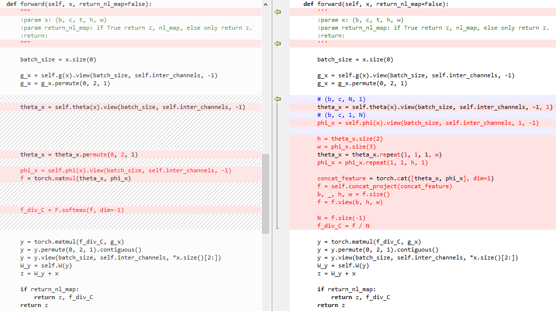
左侧为embedded Gaussian,右侧为点乘
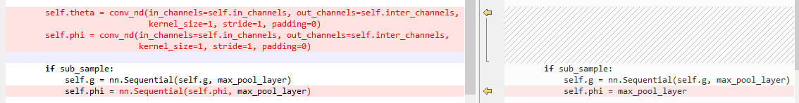
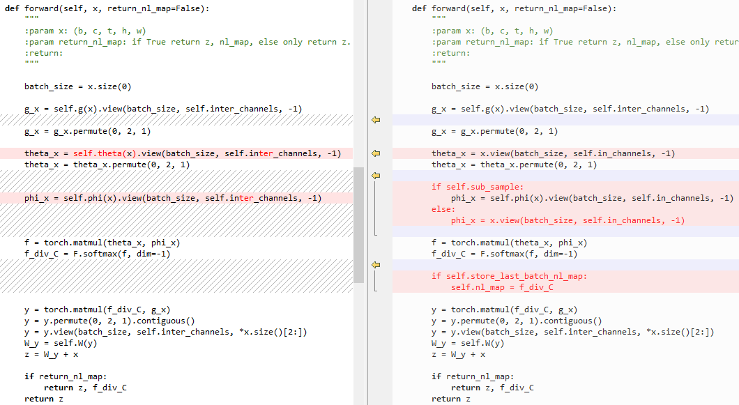
6.3 embedded Gaussian和Gaussian的区别
左侧为embedded Gaussian,右侧为Gaussian
初始化:
forward:
6.4 embedded Gaussian和Concatenation的区别
Concatenation代码:
 class _NonLocalBlockND(nn.Module):

     def __init__(self, in_channels, inter_channels=None, dimension=3, sub_sample=True, bn_layer=True):

         super(_NonLocalBlockND, self).__init__()

         assert dimension in [1, 2, 3]

         self.dimension = dimension

         self.sub_sample = sub_sample

         self.in_channels = in_channels

         self.inter_channels = inter_channels

         if self.inter_channels is None:

             self.inter_channels = in_channels // 2

             if self.inter_channels == 0:

                 self.inter_channels = 1

         if dimension == 3:

             conv_nd = nn.Conv3d

             max_pool_layer = nn.MaxPool3d(kernel_size=(1, 2, 2))

             bn = nn.BatchNorm3d

         elif dimension == 2:

             conv_nd = nn.Conv2d

             max_pool_layer = nn.MaxPool2d(kernel_size=(2, 2))

             bn = nn.BatchNorm2d

         else:

             conv_nd = nn.Conv1d

             max_pool_layer = nn.MaxPool1d(kernel_size=(2))

             bn = nn.BatchNorm1d

         self.g = conv_nd(in_channels=self.in_channels, out_channels=self.inter_channels,

                          kernel_size=1, stride=1, padding=0)

         if bn_layer:

             self.W = nn.Sequential(

                 conv_nd(in_channels=self.inter_channels, out_channels=self.in_channels,

                         kernel_size=1, stride=1, padding=0),

                 bn(self.in_channels)

             )

             nn.init.constant_(self.W[1].weight, 0)

             nn.init.constant_(self.W[1].bias, 0)

         else:

             self.W = conv_nd(in_channels=self.inter_channels, out_channels=self.in_channels,

                              kernel_size=1, stride=1, padding=0)

             nn.init.constant_(self.W.weight, 0)

             nn.init.constant_(self.W.bias, 0)

         self.theta = conv_nd(in_channels=self.in_channels, out_channels=self.inter_channels,

                              kernel_size=1, stride=1, padding=0)

         self.phi = conv_nd(in_channels=self.in_channels, out_channels=self.inter_channels,

                            kernel_size=1, stride=1, padding=0)

         self.concat_project = nn.Sequential(   # 将concat后的特征降维到1维的矩阵

             nn.Conv2d(self.inter_channels * 2, 1, 1, 1, 0, bias=False),

             nn.ReLU()

         )

         if sub_sample:

             self.g = nn.Sequential(self.g, max_pool_layer)

             self.phi = nn.Sequential(self.phi, max_pool_layer)

     def forward(self, x, return_nl_map=False):

         '''

         :param x: (b, c, t, h, w)

         :param return_nl_map: if True return z, nl_map, else only return z.

         :return:

         '''

         # 令x维度B*C*(K):一维时,x为B*C*(K1);二维时,x为B*C*(K1*K2);三维时,x为B*C*(K1*K2*K3)

         batch_size = x.size(0)

         g_x = self.g(x).view(batch_size, self.inter_channels, -1)   # 通过g函数,并reshape,得到B*inter_channels*(K)矩阵

         g_x = g_x.permute(0, 2, 1)  # 得到B*(K)*inter_channels矩阵,和图2中一致

         # (b, c, N, 1)

         theta_x = self.theta(x).view(batch_size, self.inter_channels, -1, 1)  # 通过θ函数,并reshape,得到B*inter_channels*(K)*1矩阵

         # (b, c, 1, N)

         phi_x = self.phi(x).view(batch_size, self.inter_channels, 1, -1) # 通过φ函数,并reshape,得到B*inter_channels*1*(K)矩阵

         h = theta_x.size(2)  # (K)

         w = phi_x.size(3)  # (K)

         theta_x = theta_x.repeat(1, 1, 1, w)  # B*inter_channels*(K)*(K)

         phi_x = phi_x.repeat(1, 1, h, 1)     # B*inter_channels*(K)*(K)

         concat_feature = torch.cat([theta_x, phi_x], dim=1)  # B*(2*inter_channels)*(K)*(K)

         f = self.concat_project(concat_feature)    # B*1*(K)*(K)

         b, _, h, w = f.size()  # B,_,(K),(K)

         f = f.view(b, h, w)   # B*(K)*(K)

         N = f.size(-1)  # (K)

         f_div_C = f / N   # 最后一维归一化,B*(K)*(K)

         y = torch.matmul(f_div_C, g_x)    # 得到B*(K)*inter_channels矩阵,和图2中一致

         y = y.permute(0, 2, 1).contiguous()# 得到B*inter_channels*(K)矩阵,和图2中一致

         y = y.view(batch_size, self.inter_channels, *x.size()[2:])  # 得到B*inter_channels*(K1或K1*K2或K1*K2*K3)矩阵,和图2中一致

         W_y = self.W(y)  # 得到B*C*(K)矩阵,和图2中一致

         z = W_y + x   # 特征图和non local的图相加,得到新的特征图,B*C*(K)

         if return_nl_map:

             return z, f_div_C    # 返回结果及归一化的特征

         return z

 class NONLocalBlock1D(_NonLocalBlockND):

     def __init__(self, in_channels, inter_channels=None, sub_sample=True, bn_layer=True):

         super(NONLocalBlock1D, self).__init__(in_channels,

                                               inter_channels=inter_channels,

                                               dimension=1, sub_sample=sub_sample,

                                               bn_layer=bn_layer)

 class NONLocalBlock2D(_NonLocalBlockND):

     def __init__(self, in_channels, inter_channels=None, sub_sample=True, bn_layer=True):

         super(NONLocalBlock2D, self).__init__(in_channels,

                                               inter_channels=inter_channels,

                                               dimension=2, sub_sample=sub_sample,

                                               bn_layer=bn_layer)

 class NONLocalBlock3D(_NonLocalBlockND):

     def __init__(self, in_channels, inter_channels=None, sub_sample=True, bn_layer=True,):

         super(NONLocalBlock3D, self).__init__(in_channels,

                                               inter_channels=inter_channels,

                                               dimension=3, sub_sample=sub_sample,

                                               bn_layer=bn_layer)

 if __name__ == '__main__':

     import torch

     for (sub_sample_, bn_layer_) in [(True, True), (False, False), (True, False), (False, True)]:

         img = torch.zeros(2, 3, 20)

         net = NONLocalBlock1D(3, sub_sample=sub_sample_, bn_layer=bn_layer_)

         out = net(img)

         print(out.size())

         img = torch.zeros(2, 3, 20, 20)

         net = NONLocalBlock2D(3, sub_sample=sub_sample_, bn_layer=bn_layer_)

         out = net(img)

         print(out.size())

         img = torch.randn(2, 3, 8, 20, 20)

         net = NONLocalBlock3D(3, sub_sample=sub_sample_, bn_layer=bn_layer_)

         out = net(img)

         print(out.size())
左侧为embedded Gaussian,右侧为Concatenation
初始化:

forward:
(原)Non-local Neural Networks的更多相关文章
- Local Binary Convolutional Neural Networks ---卷积深度网络移植到嵌入式设备上?
前言:今天他给大家带来一篇发表在CVPR 2017上的文章. 原文:LBCNN 原文代码:https://github.com/juefeix/lbcnn.torch 本文主要内容:把局部二值与卷积神 ...
- Spurious Local Minima are Common in Two-Layer ReLU Neural Networks
目录 引 主要内容 定理1 推论1 引理1 引理2 Safran I, Shamir O. Spurious Local Minima are Common in Two-Layer ReLU Neu ...
- 论文解读(LA-GNN)《Local Augmentation for Graph Neural Networks》
论文信息 论文标题:Local Augmentation for Graph Neural Networks论文作者:Songtao Liu, Hanze Dong, Lanqing Li, Ting ...
- Deep Learning 16:用自编码器对数据进行降维_读论文“Reducing the Dimensionality of Data with Neural Networks”的笔记
前言 论文“Reducing the Dimensionality of Data with Neural Networks”是深度学习鼻祖hinton于2006年发表于<SCIENCE > ...
- Stanford机器学习---第五讲. 神经网络的学习 Neural Networks learning
原文 http://blog.csdn.net/abcjennifer/article/details/7758797 本栏目(Machine learning)包括单参数的线性回归.多参数的线性回归 ...
- Non-local Neural Networks
1. 摘要 卷积和循环神经网络中的操作都是一次处理一个局部邻域,在这篇文章中,作者提出了一个非局部的操作来作为捕获远程依赖的通用模块. 受计算机视觉中经典的非局部均值方法启发,我们的非局部操作计算某一 ...
- 论文解读二代GCN《Convolutional Neural Networks on Graphs with Fast Localized Spectral Filtering》
Paper Information Title:Convolutional Neural Networks on Graphs with Fast Localized Spectral Filteri ...
- 【转】Artificial Neurons and Single-Layer Neural Networks
原文:written by Sebastian Raschka on March 14, 2015 中文版译文:伯乐在线 - atmanic 翻译,toolate 校稿 This article of ...
- [转]Neural Networks, Manifolds, and Topology
colah's blog Blog About Contact Neural Networks, Manifolds, and Topology Posted on April 6, 2014 top ...
随机推荐
- 从 ListView 到 RecyclerView 的用法浅析
文章目录 要走好明天的路,必须记住昨天走过的路,思索今天正在走着的路. ListView,一种在垂直滚动列表中显示条目的视图:RecyclerView,一种在局限的窗口呈现大数据集合的灵活视图.Rec ...
- YCSB项目学习
主要总结Yahoo的数据库测试项目YCSB的使用(针对redis). github网址:https://github.com/brianfrankcooper/YCSB 需要安装 java maven ...
- Mac开发环境部署
1. 安装 Xcode command line tools xcode-select --install 2. 安装 Homebrew 安装 Homebrew 之前,必须先安装 Xcode Comm ...
- 云机器同步数据 - rsync
一.需求 从google cloud云机器上定期同步图片内容,选用了支持增量备份的rsync. 二.rsync概述 rsyn是类unix系统下的数据镜像备份工具 - remote sync,安全性高, ...
- JavaScript学习总结之数组常用的方法和属性
先点赞后关注,防止会迷路寄语:没有一个冬天不会过去,没有一个春天不会到来. 前言数组常用的属性和方法常用属性返回数组的大小常用方法栈方法队列方法重排序方法操作方法转换方法迭代方法归并方法总结结尾 前言 ...
- 何用Java8 Stream API进行数据抽取与收集
上一篇中我们通过一个实例看到了Java8 Stream API 相较于传统的的Java 集合操作的简洁与优势,本篇我们依然借助于一个实际的例子来看看Java8 Stream API 如何抽取及收集数据 ...
- Linux-基本操作(登入登出,图形化界面,命令行界面)
命令行界面登录 (1)命令行登录界面 安装好Centos后,系统启动默认进入的是图形化界面,可以通过如下命令修改进入命令行界面: 命令行登录:systemctl set-default multi ...
- FCC 成都社区·前端周刊 第 7 期
01. ES2016, 2017, 2018 中的新特性 文章介绍了 18 个 ECMAScript 2016,2017 和 2018 中新增加的特性,这些特性已被加入到 TC39 提案中.包括Arr ...
- A. New Building for SIS Codeforce
You are looking at the floor plan of the Summer Informatics School's new building. You were tasked w ...
- springcloud eureka注册中心搭建
环境描述 ① jdk1.8 ② idea ③ springcloud版本 Finchley.SR2 ④ maven3.0+ 导入jar包 <properties> <project. ...