
Factoextra R Package: Easy Multivariate Data Analyses and Elegant Visualization
factoextra is an R package making easy to extract and visualize the output of exploratory multivariate data analyses, including:
Principal Component Analysis (PCA), which is used to summarize the information contained in a continuous (i.e, quantitative) multivariate data by reducing the dimensionality of the data without loosing important information.
Correspondence Analysis (CA), which is an extension of the principal component analysis suited to analyse a large contingency table formed by two qualitative variables (or categorical data).
Multiple Correspondence Analysis (MCA), which is an adaptation of CA to a data table containing more than two categorical variables.
Multiple Factor Analysis (MFA) dedicated to datasets where variables are organized into groups (qualitative and/or quantitative variables).
Hierarchical Multiple Factor Analysis (HMFA): An extension of MFA in a situation where the data are organized into a hierarchical structure.
Factor Analysis of Mixed Data (FAMD), a particular case of the MFA, dedicated to analyze a data set containing both quantitative and qualitative variables.
There are a number of R packages implementing principal component methods. These packages include: FactoMineR, ade4,stats, ca, MASS and ExPosition.
However, the result is presented differently according to the used packages. To help in the interpretation and in the visualization of multivariate analysis - such as cluster analysis and dimensionality reduction analysis - we developed an easy-to-use R package named factoextra.
The R package factoextra has flexible and easy-to-use methods to extract quickly, in a human readable standard data format, the analysis results from the different packages mentioned above.
It produces a ggplot2-based elegant data visualization with less typing.
- It contains also many functions facilitating clustering analysis and visualization.
We’ll use i) the FactoMineR package (Sebastien Le, et al., 2008) to compute PCA, (M)CA, FAMD, MFA and HCPC; ii) and the factoextra package for extracting and visualizing the results.
FactoMineR is a great and my favorite package for computing principal component methods in R. It’s very easy to use and very well documented. The official website is available at: http://factominer.free.fr/. Thanks to François Husson for his impressive work.
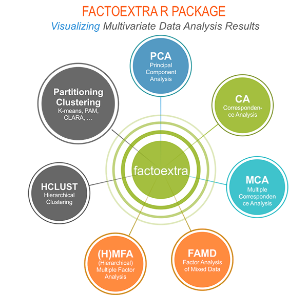
The figure below shows methods, which outputs can be visualized using the factoextra package. The official online documentation is available at: http://www.sthda.com/english/rpkgs/factoextra.
Why using factoextra?
The factoextra R package can handle the results of PCA, CA, MCA, MFA, FAMD and HMFA from several packages, for extracting and visualizing the most important information contained in your data.
- After PCA, CA, MCA, MFA, FAMD and HMFA, the most important row/column elements can be highlighted using :
- their cos2 values corresponding to their quality of representation on the factor map
- their contributions to the definition of the principal dimensions.
If you want to do this, the factoextra package provides a convenient solution.
- PCA and (M)CA are used sometimes for prediction problems : one can predict the coordinates of new supplementary variables (quantitative and qualitative) and supplementary individuals using the information provided by the previously performed PCA or (M)CA. This can be done easily using the FactoMineR package.
If you want to make predictions with PCA/MCA and to visualize the position of the supplementary variables/individuals on the factor map using ggplot2: then factoextra can help you. It’s quick, write less and do more…
- Several functions from different packages - FactoMineR, ade4, ExPosition, stats - are available in R for performing PCA, CA or MCA. However, The components of the output vary from package to package.
No matter the package you decided to use, factoextra can give you a human understandable output.
Installing FactoMineR
The FactoMineR package can be installed and loaded as follow:
# Install

install.packages("FactoMineR")

# Load

library("FactoMineR")
Installing and loading factoextra
- factoextra can be installed from CRAN as follow:
install.packages("factoextra")- Or, install the latest version from Github
if(!require(devtools)) install.packages("devtools")

devtools::install_github("kassambara/factoextra")- Load factoextra as follow :
library("factoextra")Main functions in the factoextra package
See the online documentation (http://www.sthda.com/english/rpkgs/factoextra) for a complete list.
Visualizing dimension reduction analysis outputs
| Functions | Description |
|---|---|
| fviz_eig (or fviz_eigenvalue) | Extract and visualize the eigenvalues/variances of dimensions. |
| fviz_pca | Graph of individuals/variables from the output of Principal Component Analysis (PCA). |
| fviz_ca | Graph of column/row variables from the output of Correspondence Analysis (CA). |
| fviz_mca | Graph of individuals/variables from the output of Multiple Correspondence Analysis (MCA). |
| fviz_mfa | Graph of individuals/variables from the output of Multiple Factor Analysis (MFA). |
| fviz_famd | Graph of individuals/variables from the output of Factor Analysis of Mixed Data (FAMD). |
| fviz_hmfa | Graph of individuals/variables from the output of Hierarchical Multiple Factor Analysis (HMFA). |
| fviz_ellipses | Draw confidence ellipses around the categories. |
| fviz_cos2 | Visualize the quality of representation of the row/column variable from the results of PCA, CA, MCA functions. |
| fviz_contrib | Visualize the contributions of row/column elements from the results of PCA, CA, MCA functions. |
Extracting data from dimension reduction analysis outputs
| Functions | Description |
|---|---|
| get_eigenvalue | Extract and visualize the eigenvalues/variances of dimensions. |
| get_pca | Extract all the results (coordinates, squared cosine, contributions) for the active individuals/variables from Principal Component Analysis (PCA) outputs. |
| get_ca | Extract all the results (coordinates, squared cosine, contributions) for the active column/row variables from Correspondence Analysis outputs. |
| get_mca | Extract results from Multiple Correspondence Analysis outputs. |
| get_mfa | Extract results from Multiple Factor Analysis outputs. |
| get_famd | Extract results from Factor Analysis of Mixed Data outputs. |
| get_hmfa | Extract results from Hierarchical Multiple Factor Analysis outputs. |
| facto_summarize | Subset and summarize the output of factor analyses. |
Clustering analysis and visualization
| Functions | Description |
|---|---|
| dist(fviz_dist, get_dist) | Enhanced Distance Matrix Computation and Visualization. |
| get_clust_tendency | Assessing Clustering Tendency. |
| fviz_nbclust(fviz_gap_stat) | Determining and Visualizing the Optimal Number of Clusters. |
| fviz_dend | Enhanced Visualization of Dendrogram |
| fviz_cluster | Visualize Clustering Results |
| fviz_mclust | Visualize Model-based Clustering Results |
| fviz_silhouette | Visualize Silhouette Information from Clustering. |
| hcut | Computes Hierarchical Clustering and Cut the Tree |
| hkmeans (hkmeans_tree, print.hkmeans) | Hierarchical k-means clustering. |
| eclust | Visual enhancement of clustering analysis |
Dimension reduction and factoextra
As depicted in the figure below, the type of analysis to be performed depends on the data set formats and structures.
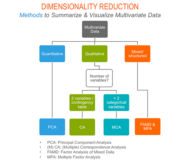
In this section we start by illustrating classical methods - such as PCA, CA and MCA - for analyzing a data set containing continuous variables, contingency table and qualitative variables, respectively.
We continue by discussing advanced methods - such as FAMD, MFA and HMFA - for analyzing a data set containing a mix of variables (qualitatives & quantitatives) organized or not into groups.
Finally, we show how to perform hierarchical clustering on principal components (HCPC), which useful for performing clustering with a data set containing only qualitative variables or with a mixed data of qualitative and quantitative variables.
Principal component analysis
- Data: decathlon2 [in factoextra package]
- PCA function: FactoMineR::PCA()
- Visualization factoextra::fviz_pca()
Read more about computing and interpreting principal component analysis at: Principal Component Analysis (PCA).
- Loading data
library("factoextra")

data("decathlon2")

df <- decathlon2[1:23, 1:10]- Principal component analysis
library("FactoMineR")

res.pca <- PCA(df, graph = FALSE)- Extract and visualize eigenvalues/variances:
# Extract eigenvalues/variances

get_eig(res.pca)
## eigenvalue variance.percent cumulative.variance.percent
## Dim.1 4.1242133 41.242133 41.24213
## Dim.2 1.8385309 18.385309 59.62744
## Dim.3 1.2391403 12.391403 72.01885
## Dim.4 0.8194402 8.194402 80.21325
## Dim.5 0.7015528 7.015528 87.22878
## Dim.6 0.4228828 4.228828 91.45760
## Dim.7 0.3025817 3.025817 94.48342
## Dim.8 0.2744700 2.744700 97.22812
## Dim.9 0.1552169 1.552169 98.78029
## Dim.10 0.1219710 1.219710 100.00000# Visualize eigenvalues/variances
fviz_screeplot(res.pca, addlabels = TRUE, ylim = c(0, 50))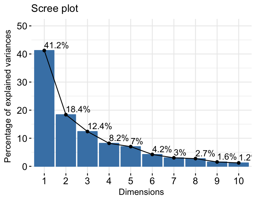
4.Extract and visualize results for variables:
# Extract the results for variables

var <- get_pca_var(res.pca)

var
## Principal Component Analysis Results for variables
## ===================================================
## Name Description
## 1 "$coord" "Coordinates for the variables"
## 2 "$cor" "Correlations between variables and dimensions"
## 3 "$cos2" "Cos2 for the variables"
## 4 "$contrib" "contributions of the variables"# Coordinates of variables
head(var$coord)## Dim.1 Dim.2 Dim.3 Dim.4 Dim.5
## X100m -0.8506257 -0.17939806 0.3015564 0.03357320 -0.1944440
## Long.jump 0.7941806 0.28085695 -0.1905465 -0.11538956 0.2331567
## Shot.put 0.7339127 0.08540412 0.5175978 0.12846837 -0.2488129
## High.jump 0.6100840 -0.46521415 0.3300852 0.14455012 0.4027002
## X400m -0.7016034 0.29017826 0.2835329 0.43082552 0.1039085
## X110m.hurdle -0.7641252 -0.02474081 0.4488873 -0.01689589 0.2242200# Contribution of variables
head(var$contrib)## Dim.1 Dim.2 Dim.3 Dim.4 Dim.5
## X100m 17.544293 1.7505098 7.338659 0.13755240 5.389252
## Long.jump 15.293168 4.2904162 2.930094 1.62485936 7.748815
## Shot.put 13.060137 0.3967224 21.620432 2.01407269 8.824401
## High.jump 9.024811 11.7715838 8.792888 2.54987951 23.115504
## X400m 11.935544 4.5799296 6.487636 22.65090599 1.539012
## X110m.hurdle 14.157544 0.0332933 16.261261 0.03483735 7.166193# Graph of variables: default plot
fviz_pca_var(res.pca, col.var = "black")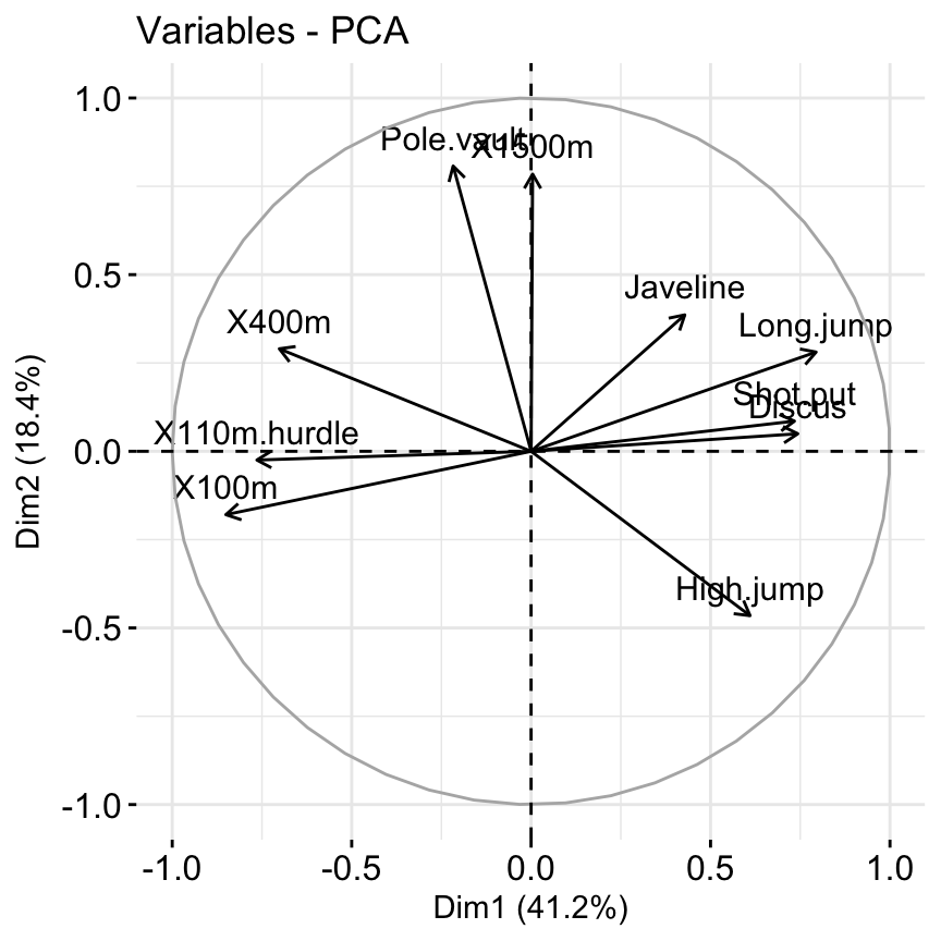
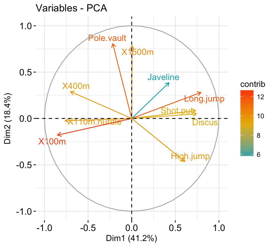
It’s possible to control variable colors using their contributions (“contrib”) to the principal axes:
# Control variable colors using their contributions

fviz_pca_var(res.pca, col.var="contrib",

             gradient.cols = c("#00AFBB", "#E7B800", "#FC4E07"),

             repel = TRUE # Avoid text overlapping

             )
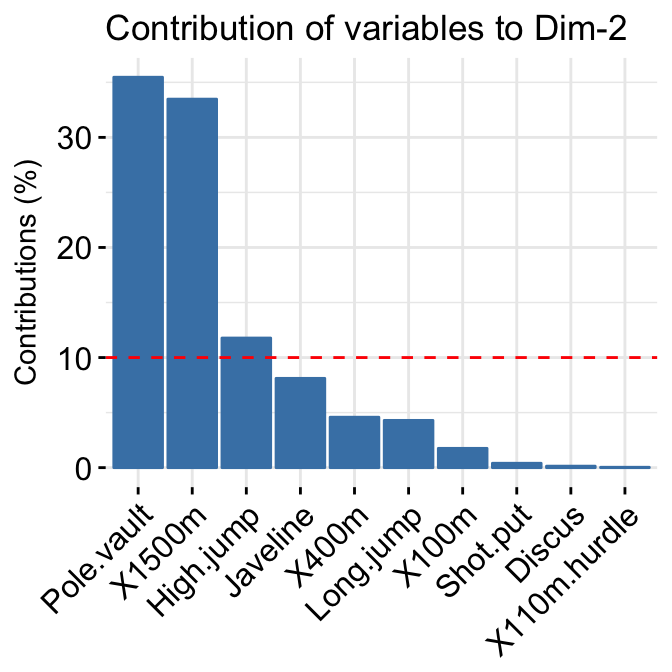
- Variable contributions to the principal axes:
# Contributions of variables to PC1

fviz_contrib(res.pca, choice = "var", axes = 1, top = 10)

# Contributions of variables to PC2

fviz_contrib(res.pca, choice = "var", axes = 2, top = 10)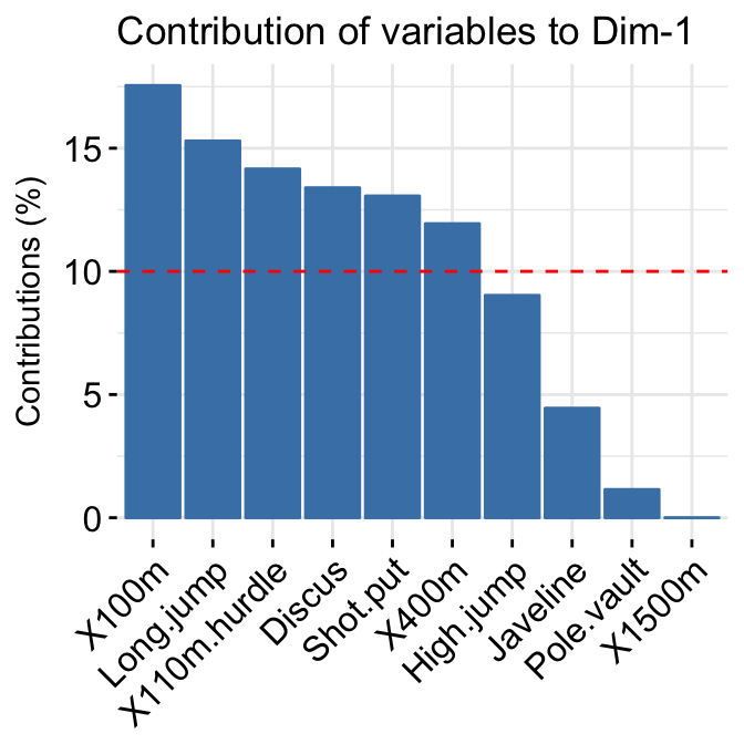
- Extract and visualize results for individuals:
# Extract the results for individuals

ind <- get_pca_ind(res.pca)

ind
## Principal Component Analysis Results for individuals
## ===================================================
## Name Description
## 1 "$coord" "Coordinates for the individuals"
## 2 "$cos2" "Cos2 for the individuals"
## 3 "$contrib" "contributions of the individuals"# Coordinates of individuals
head(ind$coord)## Dim.1 Dim.2 Dim.3 Dim.4 Dim.5
## SEBRLE 0.1955047 1.5890567 0.6424912 0.08389652 1.16829387
## CLAY 0.8078795 2.4748137 -1.3873827 1.29838232 -0.82498206
## BERNARD -1.3591340 1.6480950 0.2005584 -1.96409420 0.08419345
## YURKOV -0.8889532 -0.4426067 2.5295843 0.71290837 0.40782264
## ZSIVOCZKY -0.1081216 -2.0688377 -1.3342591 -0.10152796 -0.20145217
## McMULLEN 0.1212195 -1.0139102 -0.8625170 1.34164291 1.62151286# Graph of individuals
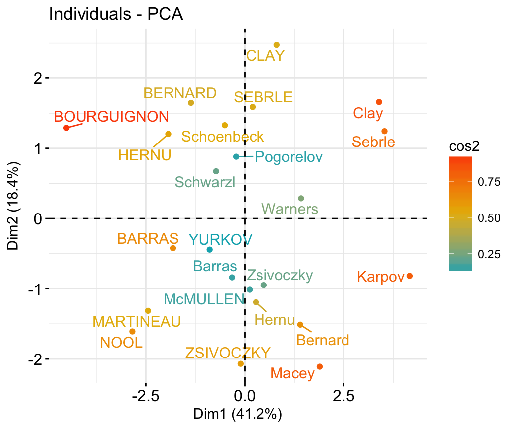
# 1. Use repel = TRUE to avoid overplotting
# 2. Control automatically the color of individuals using the cos2
# cos2 = the quality of the individuals on the factor map
# Use points only
# 3. Use gradient color
fviz_pca_ind(res.pca, col.ind = "cos2",
gradient.cols = c("#00AFBB", "#E7B800", "#FC4E07"),
repel = TRUE # Avoid text overlapping (slow if many points)
)
# Biplot of individuals and variables

fviz_pca_biplot(res.pca, repel = TRUE)
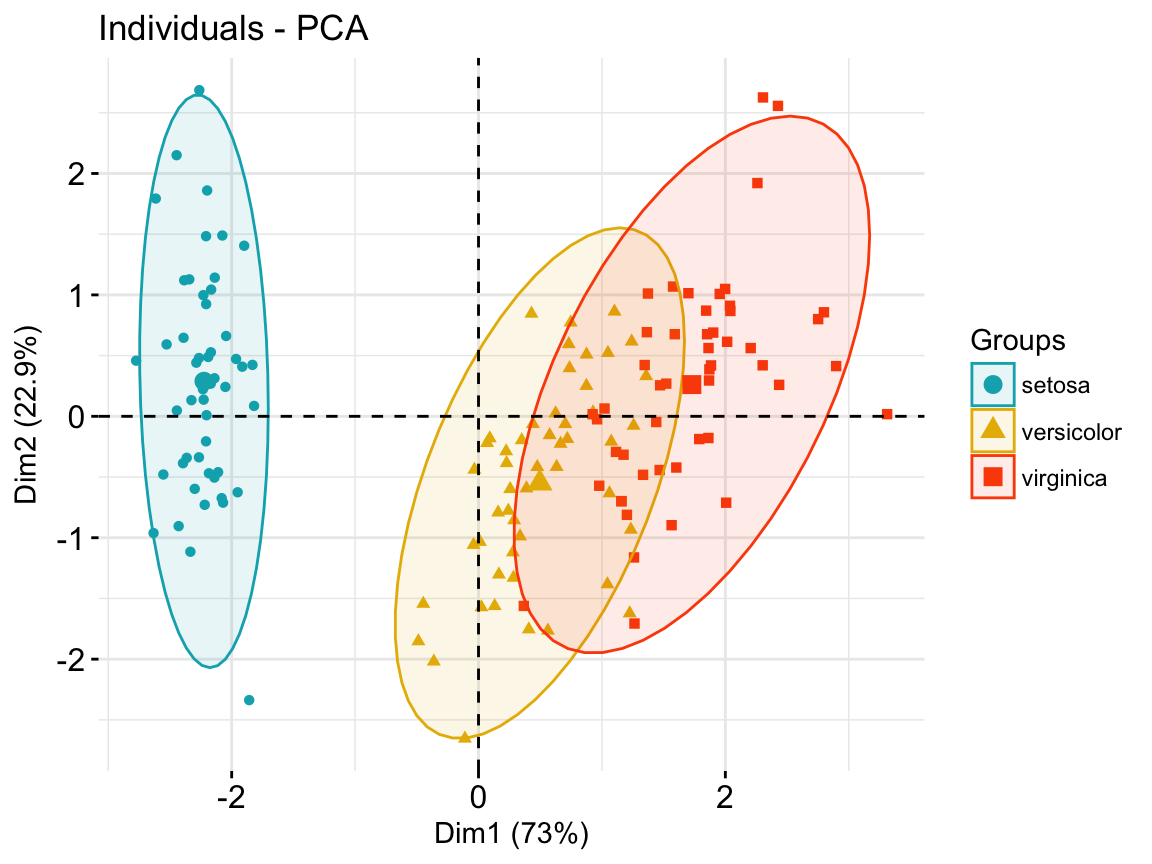
- Color individuals by groups:
# Compute PCA on the iris data set

# The variable Species (index = 5) is removed

# before PCA analysis

iris.pca <- PCA(iris[,-5], graph = FALSE)

# Visualize

# Use habillage to specify groups for coloring

fviz_pca_ind(iris.pca,

             label = "none", # hide individual labels

             habillage = iris$Species, # color by groups

             palette = c("#00AFBB", "#E7B800", "#FC4E07"),

             addEllipses = TRUE # Concentration ellipses

             )
Correspondence analysis
- Data: housetasks [in factoextra]
- CA function FactoMineR::CA()
- Visualize with factoextra::fviz_ca()
Read more about computing and interpreting correspondence analysis at: Correspondence Analysis (CA).
- Compute CA:
 # Loading data

data("housetasks")

 # Computing CA

library("FactoMineR")

res.ca <- CA(housetasks, graph = FALSE)- Extract results for row/column variables:
# Result for row variables

get_ca_row(res.ca)

# Result for column variables

get_ca_col(res.ca)- Biplot of rows and columns
fviz_ca_biplot(res.ca, repel = TRUE)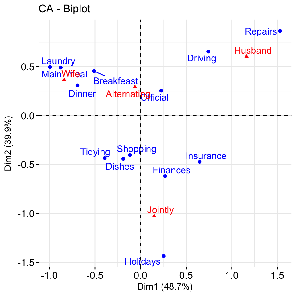
To visualize only row points or column points, type this:
# Graph of row points

fviz_ca_row(res.ca, repel = TRUE)

# Graph of column points

fviz_ca_col(res.ca)

# Visualize row contributions on axes 1

fviz_contrib(res.ca, choice ="row", axes = 1)

# Visualize column contributions on axes 1

fviz_contrib(res.ca, choice ="col", axes = 1)
Multiple correspondence analysis
- Data: poison [in factoextra]
- MCA function FactoMineR::MCA()
- Visualization factoextra::fviz_mca()
Read more about computing and interpreting multiple correspondence analysis at: Multiple Correspondence Analysis(MCA).
- Computing MCA:
library(FactoMineR)

data(poison)

res.mca <- MCA(poison, quanti.sup = 1:2,

quali.sup = 3:4, graph=FALSE)- Extract results for variables and individuals:
# Extract the results for variable categories

get_mca_var(res.mca)

# Extract the results for individuals

get_mca_ind(res.mca)- Contribution of variables and individuals to the principal axes:
# Visualize variable categorie contributions on axes 1

fviz_contrib(res.mca, choice ="var", axes = 1)

# Visualize individual contributions on axes 1

# select the top 20

fviz_contrib(res.mca, choice ="ind", axes = 1, top = 20)- Graph of individuals
# Color by groups

# Add concentration ellipses

# Use repel = TRUE to avoid overplotting

grp <- as.factor(poison[, "Vomiting"])

fviz_mca_ind(res.mca,  habillage = grp,

             addEllipses = TRUE, repel = TRUE)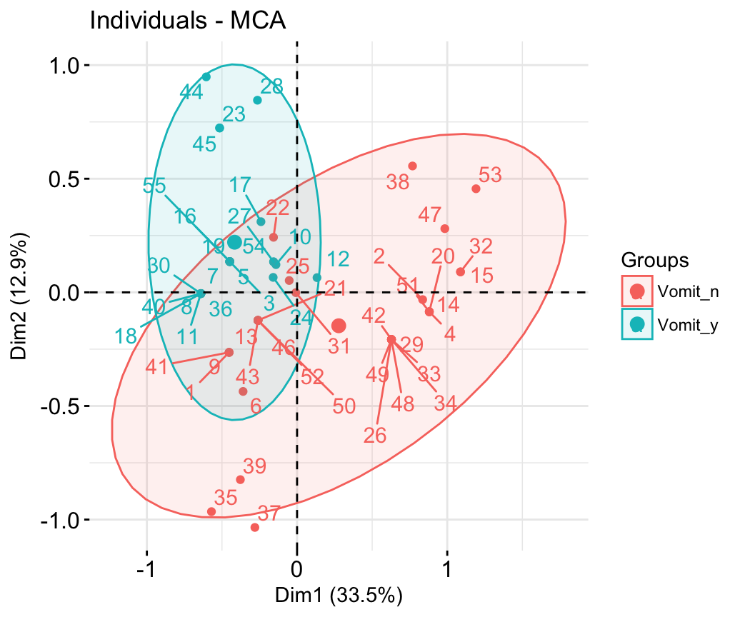
- Graph of variable categories:
fviz_mca_var(res.mca, repel = TRUE)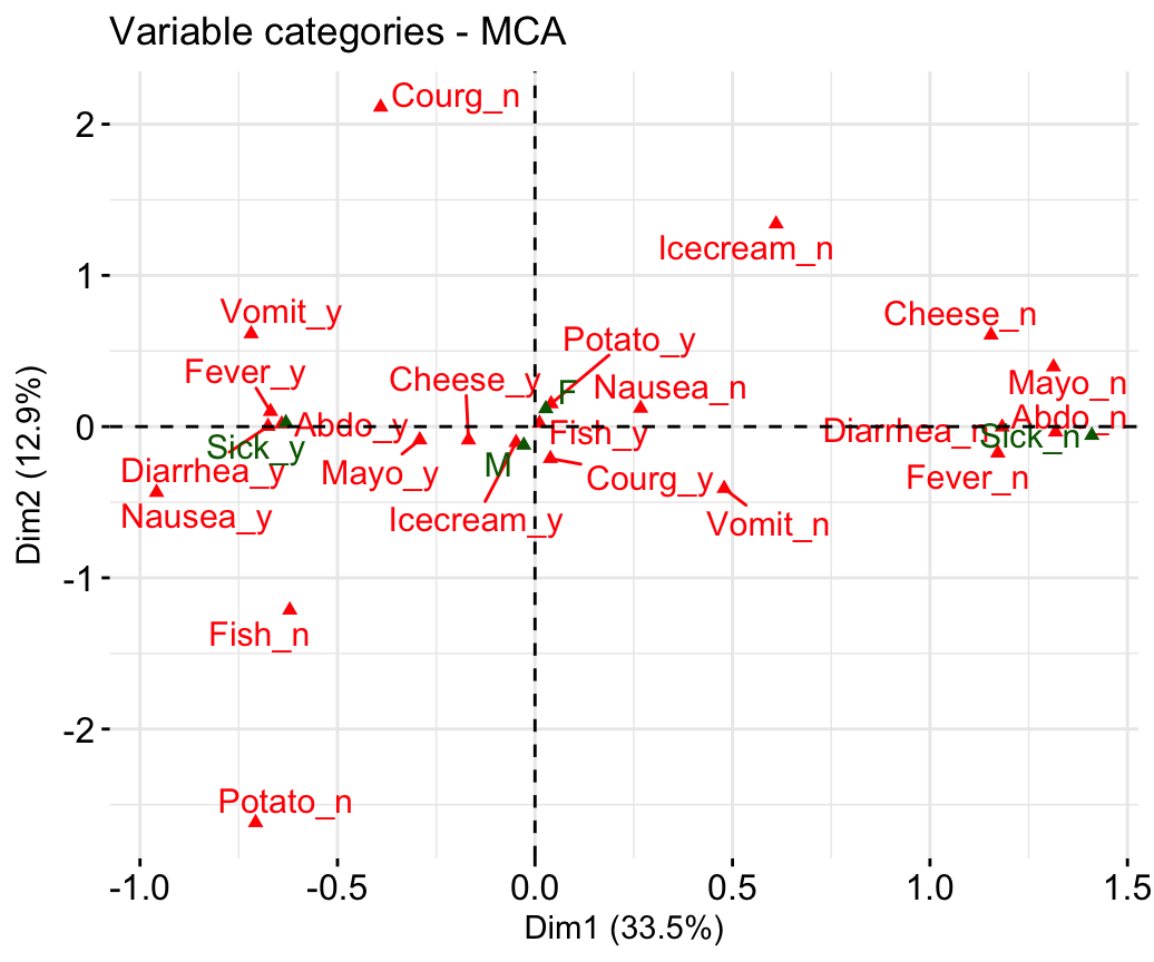
- Biplot of individuals and variables:
fviz_mca_biplot(res.mca, repel = TRUE)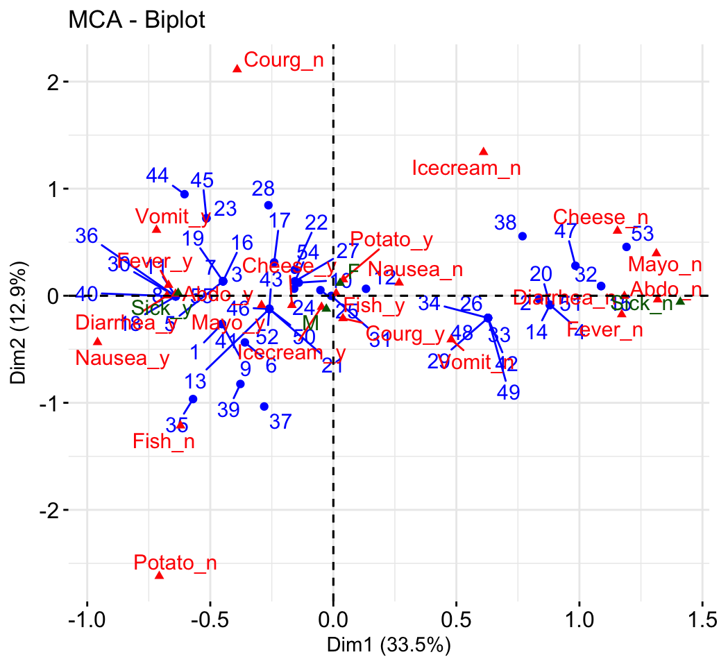
Advanced methods
The factoextra R package has also functions that support the visualization of advanced methods such:
- Factor Analysis of Mixed Data (FAMD): : FAMD Examples
- Multiple Factor Analysis (MFA): MFA Examples
- Hierarchical Multiple Factor Analysis (HMFA): HMFA Examples
- Hierachical Clustering on Principal Components (HCPC)
Cluster analysis and factoextra
To learn more about cluster analysis, you can refer to the book available at: Practical Guide to Cluster Analysis in R
The main parts of the book include:
- distance measures,
- partitioning clustering,
- hierarchical clustering,
- cluster validation methods, as well as,
- advanced clustering methods such as fuzzy clustering, density-based clustering and model-based clustering.
The book presents the basic principles of these tasks and provide many examples in R. It offers solid guidance in data mining for students and researchers.
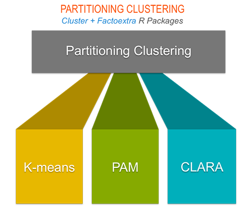
Partitioning clustering
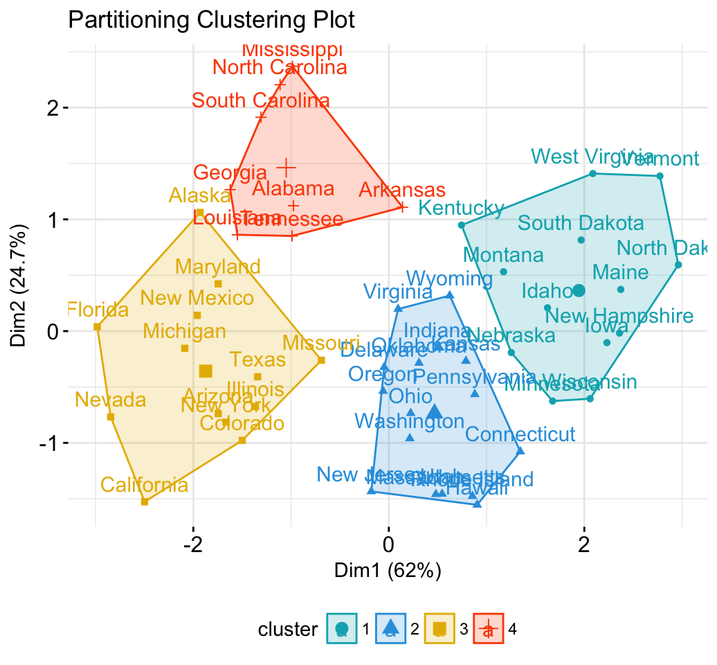
# 1. Loading and preparing data

data("USArrests")

df <- scale(USArrests)

# 2. Compute k-means

set.seed(123)

km.res <- kmeans(scale(USArrests), 4, nstart = 25)

# 3. Visualize

library("factoextra")

fviz_cluster(km.res, data = df,

             palette = c("#00AFBB","#2E9FDF", "#E7B800", "#FC4E07"),

             ggtheme = theme_minimal(),

             main = "Partitioning Clustering Plot"

             )
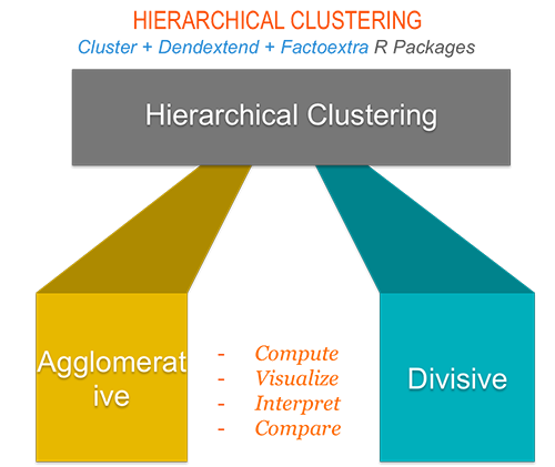
Hierarchical clustering
library("factoextra")

# Compute hierarchical clustering and cut into 4 clusters

res <- hcut(USArrests, k = 4, stand = TRUE)

# Visualize

fviz_dend(res, rect = TRUE, cex = 0.5,

          k_colors = c("#00AFBB","#2E9FDF", "#E7B800", "#FC4E07"))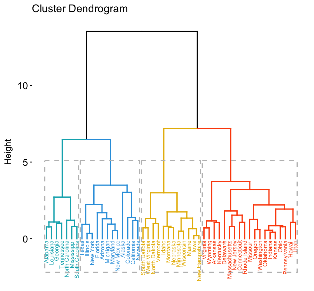
Determine the optimal number of clusters
# Optimal number of clusters for k-means

library("factoextra")

my_data <- scale(USArrests)

fviz_nbclust(my_data, kmeans, method = "gap_stat")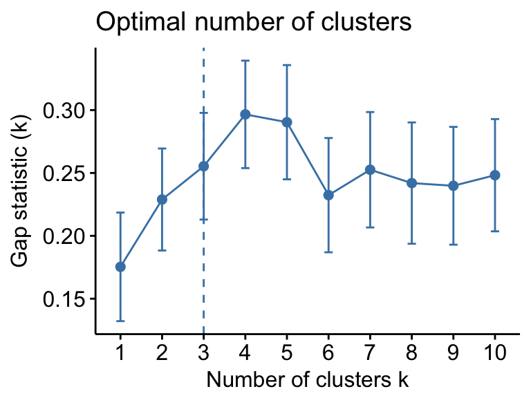
Acknoweledgment
I would like to thank Fabian Mundt for his active contributions to factoextra.
We sincerely thank all developers for their efforts behind the packages that factoextra depends on, namely, ggplot2 (Hadley Wickham, Springer-Verlag New York, 2009), FactoMineR (Sebastien Le et al., Journal of Statistical Software, 2008),dendextend (Tal Galili, Bioinformatics, 2015), cluster (Martin Maechler et al., 2016) and more …..
References
- H. Wickham (2009). ggplot2: Elegant Graphics for Data Analysis. Springer-Verlag New York.
- Maechler, M., Rousseeuw, P., Struyf, A., Hubert, M., Hornik, K.(2016). cluster: Cluster Analysis Basics and Extensions. R package version 2.0.5.
- Sebastien Le, Julie Josse, Francois Husson (2008). FactoMineR: An R Package for Multivariate Analysis. Journal of Statistical Software, 25(1), 1-18. 10.18637/jss.v025.i01
- Tal Galili (2015). dendextend: an R package for visualizing, adjusting, and comparing trees of hierarchical clustering. Bioinformatics. DOI: 10.1093/bioinformatics/btv428
转自:http://www.sthda.com/english/wiki/factoextra-r-package-easy-multivariate-data-analyses-and-elegant-visualization
Factoextra R Package: Easy Multivariate Data Analyses and Elegant Visualization的更多相关文章
- R TUTORIAL: VISUALIZING MULTIVARIATE RELATIONSHIPS IN LARGE DATASETS
In two previous blog posts I discussed some techniques for visualizing relationships involving two o ...
- 转载Quandl R Package
Quandl R Package 通过Quandl API可以快速准确地获取宏观经济数据.(https://www.quandl.com/docs/api) 分享两个国外的优秀网站 R和Python在 ...
- R语言数据分析利器data.table包 —— 数据框结构处理精讲
R语言data.table包是自带包data.frame的升级版,用于数据框格式数据的处理,最大的特点快.包括两个方面,一方面是写的快,代码简洁,只要一行命令就可以完成诸多任务,另一方面是处理 ...
- 将R非时间序列的data.frame转变为时序格式
将R非时间序列的data.frame转变为时序格式,常常会用到,尤其是股票数据处理中, 举例:dailyData包括两列数据:Date Close10/11/2013 871.9910/10/2013 ...
- R语言数据分析利器data.table包—数据框结构处理精讲
R语言数据分析利器data.table包-数据框结构处理精讲 R语言data.table包是自带包data.frame的升级版,用于数据框格式数据的处理,最大的特点快.包括两个方面,一方面是写的快,代 ...
- R︱高效数据操作——data.table包(实战心得、dplyr对比、key灵活用法、数据合并)
每每以为攀得众山小,可.每每又切实来到起点,大牛们,缓缓脚步来俺笔记葩分享一下吧,please~ --------------------------- 由于业务中接触的数据量很大,于是不得不转战开始 ...
- R读取大数据data.table包之fread
>library(data.table)>data=fread("10000000.txt")>Read 9999999 rows and 71 (of 71) ...
- R语言安装R package的2种方法
http://www.cnblogs.com/emanlee/archive/2012/12/05/2803606.html
- 基于R数据分析之常用Package讲解系列--1. data.table
利用data.table包变形数据 一. 基础概念 data.table 这种数据结构相较于R中本源的data.frame 在数据处理上有运算速度更快,内存运用更高效,可认为它是data.frame ...
随机推荐
- 常见的Java面试题整理
面试是我们每个人都要经历的事情,大部分人且不止一次,这里给大家总结常见的面试题,让大家在找工作时候能够事半功倍. 1 Switch能否用string做参数? a.在 Java 7 之前, switch ...
- Java 判断回文字符串有多少和其中的最大字符串
一.简介代码功能 该代码的功能可以实现对任意的一段字符串进行判断是否有回文,回文有哪些,和其中的最大回文. 二.代码部分 1.全局变量 static String hws = "" ...
- .NET Framework 4.7 安装
我们打开.NET Framework下载界面: https://www.microsoft.com/net/download/framework 这时你会发现,我们能下载的.NET Framework ...
- 详谈 Unity3D AssetBundle 资源加载,结合实际项目开发实例
第一次搞资源更新方面,这里只说更新,加载,AssetBundle资源加载,谈谈自己的理解,以及自己在项目中遇到的那些神坑,现在回想一下,真的是自己跪着过来的,说多了,都是泪. 我这边是安卓AssetB ...
- Redis编码问题
最近搞redis存储对象出了点问题,大概说一下背景,项目原有的东东以前存的是redis,存储的直接是对象模型,没有问题,这里存储对象存储任何信息事都没有问题的.但是现在调整为存储序列化的json字符串 ...
- 一个全局变量引起的DLL崩溃
参考我发的帖子: http://bbs.csdn.net/topics/390737064?page=1#post-397000946 现象是exe程序在加载dll的时候崩溃了,莫名其妙的崩溃了.换其 ...
- vim 字符串替换整理
公司项目测试,要在vi编辑其中进行多路径修改,这时候用到了字符串替换的知识,在这里我自己整理了一下. 一.基本内容替换,无特殊符号 :s/old/new/ 替换当前行第一个 old 为 new ...
- JS中字符串与数组的一些常用方法
真是恨透了这些类似于substring substr slice 要么长得像,要么就功能相近的方法... 1⃣️string 1.substring(start开始位置的索引,end结束位置索引) 截 ...
- jquery虎牙TV3D轮播特效
css部分: *{ margin: 0px; padding: 0px; } body{ margin: 0px; padding: 0px; text-align: center; } #banne ...
- Apache Spark1.1.0部署与开发环境搭建
Spark是Apache公司推出的一种基于Hadoop Distributed File System(HDFS)的并行计算架构.与MapReduce不同,Spark并不局限于编写map和reduce ...