Machine Learning Week_1 Model and Cost Function 5-8

目录

• 2.5 Video: Cost Function Intuition-1
  • unfamiliar words
• 2.6 Reading: Cost Function Intuition-1
  • unfamiliar words
• 2.7 Video: Cost Function Intuition-2
  • unfamiliar words
• 2.8 Reading: Cost Function Intuition-2
  • unfamiliar words

2.5 Video: Cost Function Intuition-1

In the previous video, we gave the mathematical definition of the cost function.

In this video, let's look at some examples, to get back to intuition about what the cost function is doing, and why we want to use it. To recap, here's what we had last time. We want to fit a straight line to our data, so we had this formed as a hypothesis with these parameters theta zero and theta one, and with different choices of the parameters we end up with different straight line fits. So the data which are fit like so, and there's a cost function, and that was our optimization objective.

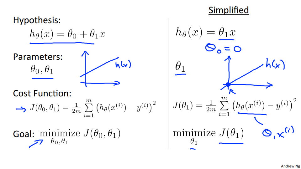
For this video, in order to better visualize the cost function J, I'm going to work with a simplified hypothesis function, like that shown on the right. So I'm gonna use my simplified hypothesis, which is just theta one times X. We can, if you want, think of this as setting the parameter theta zero equal to 0. So I have only one parameter theta one and my cost function is similar to before except that now H of X that is now equal to just theta one times X. And I have only one parameter theta one and so my optimization objective is to minimize j of theta one. In pictures what this means is that if theta zero equals zero that corresponds to choosing only hypothesis functions that pass through the origin, that pass through the point (0, 0).

Using this simplified definition of a hypothesizing cost function. Let's try to understand the cost function concept better. It turns out that two key functions we want to understand. The first is the hypothesis function, and the second is a cost function.

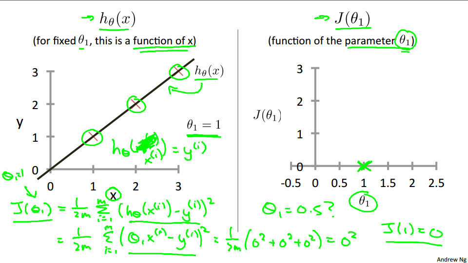
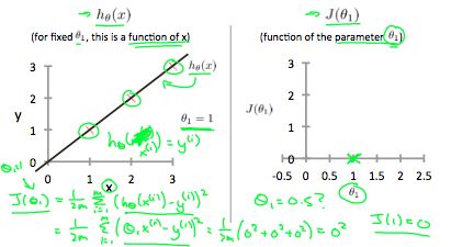
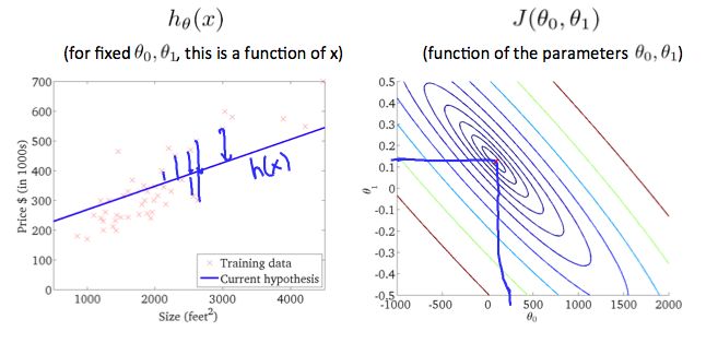
So, notice that the hypothesis, right, H of X. For a fixed value of theta one, this is a function of X. So the hypothesis is a function of, what is the size of the house X. In contrast, the cost function, J, that's a function of the parameter, theta one, which controls the slope of the straight line. Let's plot these functions and try to understand them both better.

Let's start with the hypothesis. On the left, let's say here's my training set with three points at (1, 1), (2, 2), and (3, 3). Let's pick a value theta one, so when theta one equals one, and if that's my choice for theta one, then my hypothesis is going to look like this straight line over here. And I'm gonna point out, when I'm plotting my hypothesis function. X-axis, my horizontal axis is labeled X, is labeled you know, size of the house over here. Now, of temporary, set theta one equals one, what I want to do is figure out what is j of theta one, when theta one equals one.

So let's go ahead and compute what the cost function has for the value one. Well, as usual, my cost function is defined as follows, right? Some from, some of 'em are training sets of this usual squared error term. And, this is therefore equal to. And this. Of theta one x i minus y i and if you simplify this turns out to be. That. Zero Squared to zero squared to zero squared which is of course, just equal to zero. Now, inside the cost function. It turns out each of these terms here is equal to zero. Because for the specific training set I have or my 3 training examples are (1, 1), (2, 2), (3,3). If theta one is equal to one. Then h of x. H of x i. Is equal to y i exactly, let me write this better. Right? And so, h of x minus y, each of these terms is equal to zero, which is why I find that j of one is equal to zero. So, we now know that j of one Is equal to zero. Let's plot that. What I'm gonna do on the right is plot my cost function j. And notice, because my cost function is a function of my parameter theta one, when I plot my cost function, the horizontal axis is now labeled with theta one. So I have j of one equalto zero so let's go ahead and plot that. End up with an X over there.

Now lets look at some other examples. Theta-1 can take on a range of different values. Right? So theta-1 can take on the negative values, zero, positive values. So what if theta-1 is equal to 0.5. What happens then?

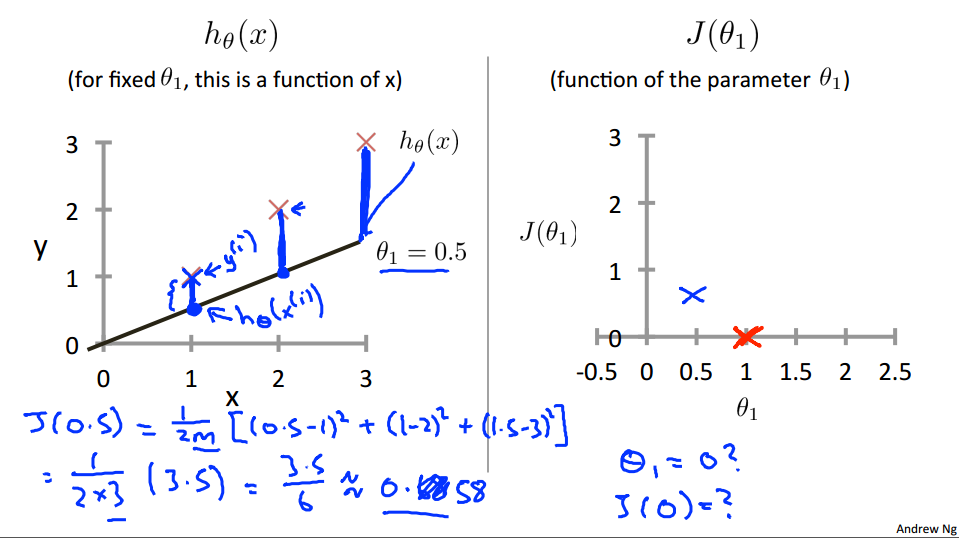
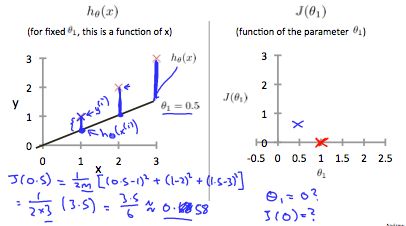
Let's go ahead and plot that. I'm now going to set theta-1 equals 0.5, and in that case my hypothesis now looks like this. As a line with slope equals to 0.5, and, lets compute J, of 0.5. So that is going to be one over 2M of, my usual cost function. It turns out that the cost function is going to be the sum of square values of the height of this line. Plus the sum of square of the height of that line, plus the sum of square of the height of that line, right? Cause just this vertical distance, that's the difference between, you know, y i and the predicted value, H of x i, right? So the first example is going to be 0.5 minus one squared. Because my hypothesis predicted 0.5. Whereas, the actual value was one. For my second example, I get, one minus two squared, because my hypothesis predicted one, but the actual housing price was two. And then finally, plus. 1.5 minus three squared. And so that's equal to one over two times three. Because, M when training set size, right, have three training examples. In that, that's times simplifying for the parentheses it's 3.5. So that's 3.5 over six which is about 0.68. So now we know that j of 0.5 is about 0.68.[Should be 0.58] Lets go and plot that. Oh excuse me, math error, it's actually 0.58. So we plot that which is maybe about over there. Okay?

Now, let's do one more. How about if theta one is equal to zero, what is J of zero equal to? It turns out that if theta one is equal to zero, then H of X is just equal to, you know, this flat line, right, that just goes horizontally like this. And so, measuring the errors. We have that J of zero is equal to one over two M, times one squared plus two squared plus three squared, which is, One over six times fourteen which is about 2.3. So let's go ahead and plot as well. So it ends up with a value around 2.3 and of course we can keep on doing this for other values of theta one.

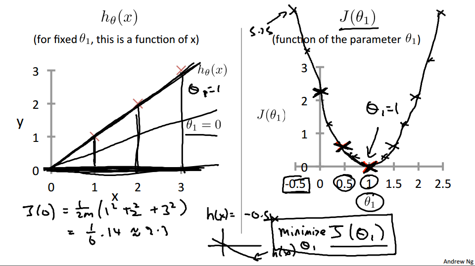
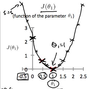
It turns out that you can have you know negative values of theta one as well so if theta one is negative then h of x would be equal to say minus 0.5 times x then theta one is minus 0.5 and so that corresponds to a hypothesis with a slope of negative 0.5. And you can actually keep on computing these errors. This turns out to be, you know, for 0.5, it turns out to have really high error. It works out to be something, like, 5.25. And so on, and the different values of theta one, you can compute these things, right? And it turns out that you, your computed range of values, you get something like that. And by computing the range of values, you can actually slowly create out. What does function J of Theta say and that's what J of Theta is. To recap, for each value of theta one, right? Each value of theta one corresponds to a different hypothesis, or to a different straight line fit on the left. And for each value of theta one, we could then derive a different value of j of theta one. And for example, you know, theta one=1, corresponded to this straight line straight through the data. Whereas theta one=0.5. And this point shown in magenta corresponded to maybe that line, and theta one=zero which is shown in blue that corresponds to this horizontal line. Right, so for each value of theta one we wound up with a different value of J of theta one and we could then use this to trace out this plot on the right.

Now you remember, the optimization objective for our learning algorithm is we want to choose the value of theta one. That minimizes J of theta one. Right? This was our objective function for the linear regression. Well, looking at this curve, the value that minimizes j of theta one is, you know, theta one equals to one. And low and behold, that is indeed the best possible straight line fit through our data, by setting theta one equals one. And just, for this particular training set, we actually end up fitting it perfectly.

And that's why minimizing j of theta one corresponds to finding a straight line that fits the data well. So, to wrap up. In this video, we looked up some plots. To understand the cost function. To do so, we simplify the algorithm. So that it only had one parameter theta one. And we set the parameter theta zero to be only zero. In the next video. We'll go back to the original problem formulation and look at some visualizations involving both theta zero and theta one. That is without setting theta zero to zero. And hopefully that will give you, an even better sense of what the cost function j is doing in the original linear regression formulation.

unfamiliar words

there's a cost function, and that was our optimization objective.

think of this as setting the parameter theta zero equal to 0.

Using this simplified definition of a hypothesizing cost function.

In that, that's times simplifying for the parentheses it's 3.5.

And this point shown in magenta corresponded to maybe that line

We'll go back to the original problem formulation and look at some visualizations involving both theta zero and theta one.

2.6 Reading: Cost Function Intuition-1

If we try to think of it in visual terms, our training data set is scattered on the x-y plane. We are trying to make a straight line (defined by \(h_{\theta}(x)\)) which passes through these scattered data points.

Our objective is to get the best possible line. The best possible line will be such so that the average squared vertical distances of the scattered points from the line will be the least. Ideally, the line should pass through all the points of our training data set. In such a case, the value of \(J(\theta_{0},\theta_{1})\) will be 0. The following example shows the ideal situation where we have a cost function of 0.

When \(\theta_{1} = 1\) we get a slope of 1 which goes through every single data point in our model. Conversely, when \(\theta_{1} = 0.5\) we see the vertical distance from our fit to the data points increase.

This increases our cost function to 0.58. Plotting several other points yields to the following graph:

Thus as a goal, we should try to minimize the cost function. In this case, \(\theta_1 = 1\) is our global minimum.

unfamiliar words

If we try to think of it in visual terms, our training data set is scattered on the x-y plane.

The following example shows the ideal situation where we have a cost function of 0.

Conversely, when \(\theta_{1} = 0.5\) we see the vertical distance from our fit to the data points increase.

2.7 Video: Cost Function Intuition-2

In this video, lets delve deeper and get even better intuition about what the cost function is doing. This video assumes that you're familiar with contour plots. If you are not familiar with contour plots or contour figures some of the illustrations in this video may or may not make sense to you but is okay and if you end up skipping this video or some of it does not quite make sense because you haven't seen contour plots before. That's okay and you will still understand the rest of this course without those parts of this.

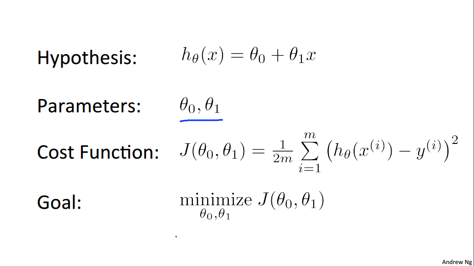
Here's our problem formulation as usual, with the hypothesis parameters, cost function, and our optimization objective.

Unlike before, unlike the last video, I'm going to keep both of my parameters, theta zero, and theta one, as we generate our visualizations for the cost function. So, same as last time, we want to understand the hypothesis H and the cost function J. So, here's my training set of housing prices and let's make some hypothesis. You know, like that one, this is not a particularly good hypothesis.

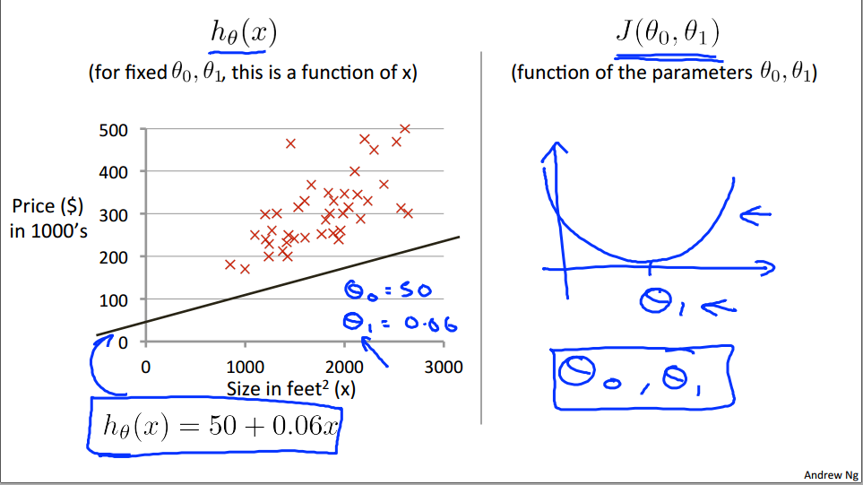
But, if I set theta zero=50 and theta one=0.06, then I end up with this hypothesis down here and that corresponds to that straight line. Now given these value of theta zero and theta one, we want to plot the corresponding, you know, cost function on the right. What we did last time was, right, when we only had theta one. In other words, drawing plots that look like this as a function of theta one.

But now we have two parameters, theta zero, and theta one, and so the plot gets a little more complicated. It turns out that when we have only one parameter, that the parts we drew had this sort of bow shaped function. Now, when we have two parameters, it turns out the cost function also has a similar sort of bow shape. And, in fact, depending on your training set, you might get a cost function that maybe looks something like this. So, this is a 3-D surface plot, where the axes are labeled theta zero and theta one.

[a static 3D image]

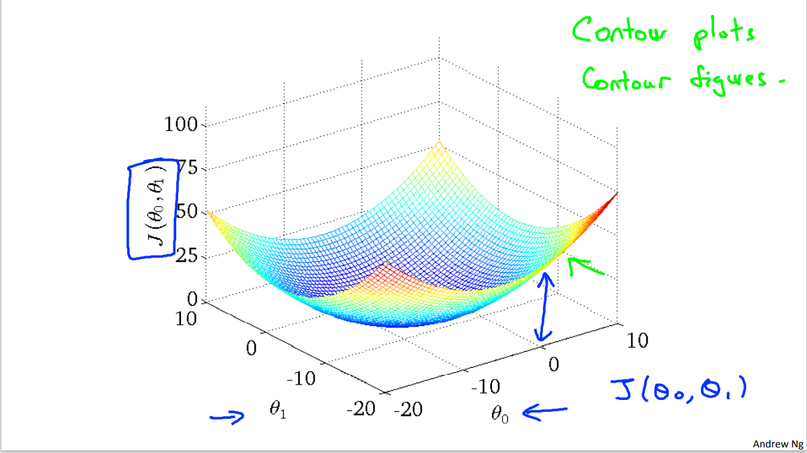
So as you vary theta zero and theta one, the two parameters, you get different values of the cost function J (theta zero, theta one) and the height of this surface above a particular point of theta zero, theta one. Right, that's, that's the vertical axis. The height of the surface of the points indicates the value of J of theta zero, J of theta one. And you can see it sort of has this bow like shape. Let me show you the same plot in 3D. So here's the same figure in 3D, horizontal axis theta one and vertical axis J(theta zero, theta one), and if I rotate this plot around. You kinda of a get a sense, I hope, of this bowl shaped surface as that's what the cost function J looks like.(At this time, the teacher left the PPT. Open the previous 3D image and rotate it.)

Now for the purpose of illustration in the rest of this video I'm not actually going to use these sort of 3D surfaces to show you the cost function J, instead I'm going to use contour plots. Or what I also call contour figures. I guess they mean the same thing. To show you these surfaces.

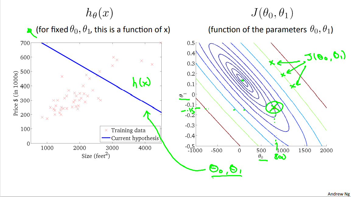
So here's an example of a contour figure, shown on the right, where the axis are theta zero and theta one. And what each of these ovals, what each of these ellipsis shows is a set of points that takes on the same value for J(theta zero, theta one). So concretely, for example this, you'll take that point and that point and that point. All three of these points that I just drew in magenta, they have the same value for J (theta zero, theta one). Okay. Where, right, these, this is the theta zero, theta one axis but those three have the same Value for J (theta zero, theta one) and if you haven't seen contour plots much before think of, imagine if you will. A bow shaped function that's coming out of my screen. So that the minimum, so the bottom of the bow is this point right there, right? This middle, the middle of these concentric ellipses. And imagine a bow shape that sort of grows out of my screen like this, so that each of these ellipses, you know, has the same height above my screen. And the minimum with the bow, right, is right down there. And so the contour figures is a, is a way to, is maybe a more convenient way to visualize my function J.

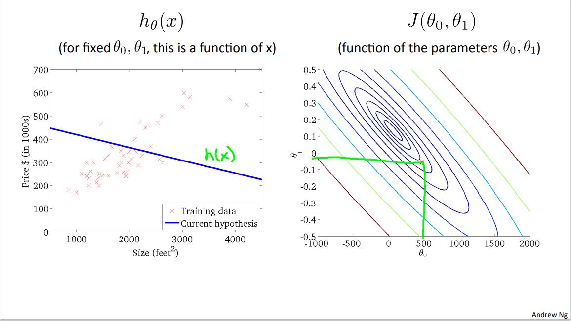
So, let's look at some examples. Over here, I have a particular point, right? And so this is, with, you know, theta zero equals maybe about 800, and theta one equals maybe a -0.15 . And so this point, right, this point in red corresponds to one set of pair values of theta zero, theta one and the corresponding, in fact, to that hypothesis, right, theta zero is about 800, that is, where it intersects the vertical axis is around 800, and this is slope of about -0.15. Now this line is really not such a good fit to the data, right. This hypothesis, h(x), with these values of theta zero, theta one, it's really not such a good fit to the data. And so you find that, it's cost. Is a value that's out here that's you know pretty far from the minimum right it's pretty far this is a pretty high cost because this is just not that good a fit to the data.

In this video, lets delve deeper and get even better intuition about what the cost function is doing.

If you are not familiar with contour plots or contour figures some of the illustrations in this video may or may not make sense to you but is okay and if you end up skipping this video or some of it does not quite make sense because you haven't seen contour plots before.

where the axes are labeled theta zero and theta one.

and if I rotate this plot around.

where the axis are theta zero and theta one. And what each of these ovals, what each of these ellipsis shows is a set of points that takes on the same value for J(theta zero, theta one).

This middle, the middle of these concentric ellipses.

where it intersects the vertical axis is around 800

is maybe a more convenient way to visualize my function J.

Let's look at some more examples. Now here's a different hypothesis that's you know still not a great fit for the data but may be slightly better so here right that's my point that those are my parameters theta zero theta one and so my theta zero value. Right?

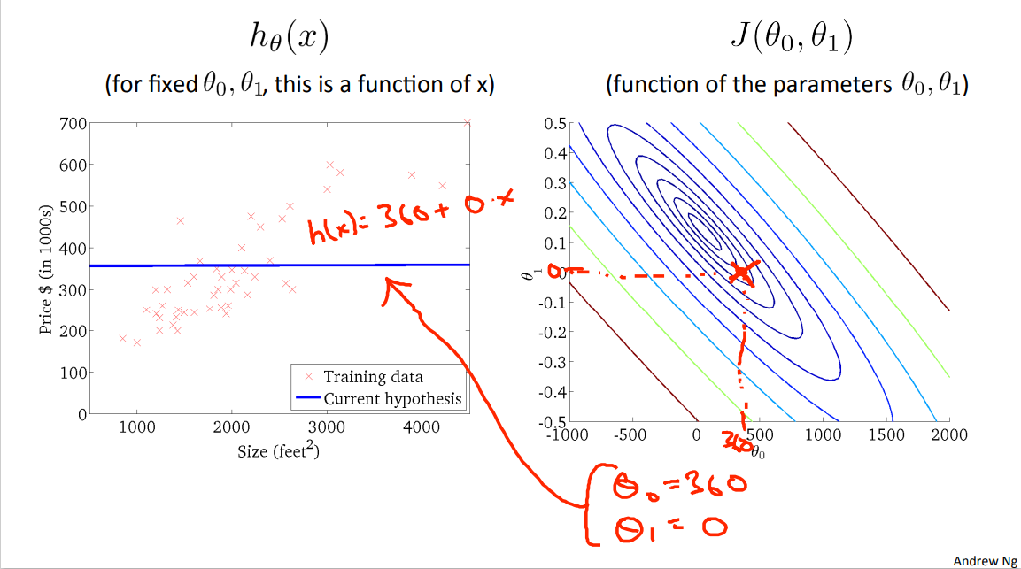
That's bout 360 and my value for theta one. Is equal to zero. So, you know, let's break it out. Let's take theta zero equals 360 theta one equals zero. And this pair of parameters corresponds to that hypothesis, corresponds to flat line, that is, h(x) equals 360 plus zero times x. So that's the hypothesis. And this hypothesis again has some cost, and that cost is, you know, plotted as the height of the J function at that point.

Let's look at just a couple of examples. Here's one more, you know, at this value of theta zero, and at that value of theta one, we end up with this hypothesis, h(x) and again, not a great fit to the data, and is actually further away from the minimum.

Last example, this is actually not quite at the minimum, but it's pretty close to the minimum. So this is not such a bad fit to the, to the data, where, for a particular value, of, theta zero. Which, one of them has value, as in for a particular value for theta one. We get a particular h(x). And this is, this is not quite at the minimum, but it's pretty close. And so the sum of squares errors is sum of squares distances between my, training samples and my hypothesis. Really, that's a sum of square distances, right? Of all of these errors. This is pretty close to the minimum even though it's not quite the minimum.

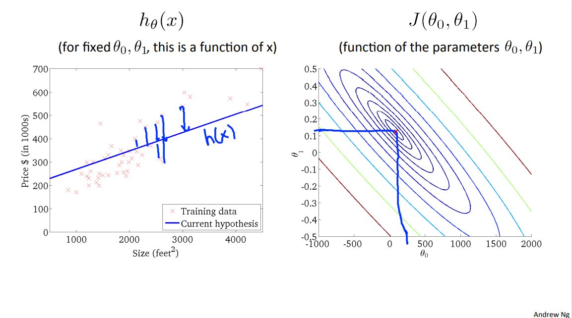
So with these figures I hope that gives you a better understanding of what values of the cost function J, how they are and how that corresponds to different hypothesis and so as how better hypotheses may corresponds to points that are closer to the minimum of this cost function J.

Now of course what we really want is an efficient algorithm, right, a efficient piece of software for automatically finding The value of theta zero and theta one, that minimizes the cost function J, right? And what we, what we don't wanna do is to, you know, how to write software, to plot out this point, and then try to manually read off the numbers, that this is not a good way to do it. And, in fact, we'll see it later, that when we look at more complicated examples, we'll have high dimensional figures with more parameters, that, it turns out, we'll see in a few, we'll see later in this course, examples where this figure, you know, cannot really be plotted, and this becomes much harder to visualize. And so, what we want is to have software to find the value of theta zero, theta one that minimizes this function and in the next video we start to talk about an algorithm for automatically finding that value of theta zero and theta one that minimizes the cost function J.

unfamiliar words

2.8 Reading: Cost Function Intuition-2

A contour plot is a graph that contains many contour lines. A contour line of a two variable function has a constant value at all points of the same line. An example of such a graph is the one to the right below.

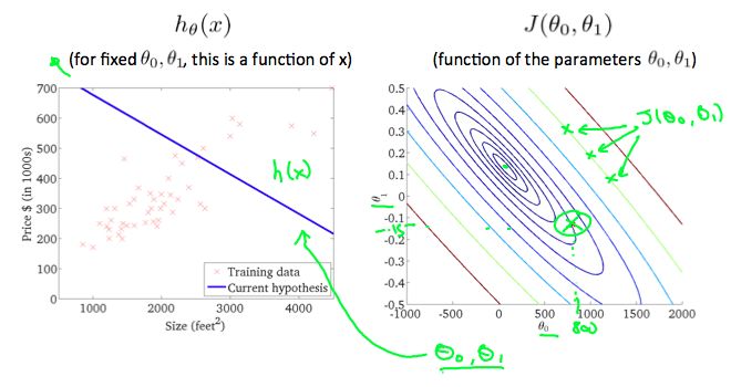
Taking any color and going along the 'circle', one would expect to get the same value of the cost function. For example, the three green points found on the green line above have the same value for \(J(\theta_{0},\theta_{1})\) and as a result, they are found along the same line. The circled x displays the value of the cost function for the graph on the left when \(\theta_{0} = 800\) and \(\theta_{1} = -0.15\) . Taking another h(x) and plotting its contour plot, one gets the following graphs:

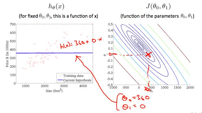
When \(\theta_{0} = 360\) and \(\theta_{1} = 0\) , the value of \(J(\theta_{0},\theta_{1})\) in the contour plot gets closer to the center thus reducing the cost function error. Now giving our hypothesis function a slightly positive slope results in a better fit of the data.

The graph above minimizes the cost function as much as possible, And consequently, the result of \(\theta_{0}\) and \(\theta_{1}\) tend to be around 0.12 and 250 respectively. Plotting those values on our graph to the right seems to put our point in the center of the inner most 'circle'.

unfamiliar words

The graph above minimizes the cost function as much as possible, And consequently, the result of \(\theta_{0}\) and \(\theta_{1}\) tend to be around 0.12 and 250 respectively.