使用Jupter Notebook实现简单的神经网络

参考：http://python.jobbole.com/82208/

注：1）# %matplotlib inline 注解可以使Jupyter中显示图片

2）注意包的导入方式

一、使用的Python包

　　1）numpy

　　　　numpy（Numerical Python）提供了python对多维数组对象的支持：ndarray，具有矢量运算能力，快速、节省空间。numpy支持高级大量的维度数组与矩阵运算，此外也针对数组运算提供大量的数学函数库。

　　　　参考：http://blog.csdn.net/cxmscb/article/details/54583415

　　2）sklearn

　　　　机器学习的一个实用工具，提供了数据集，数据预处理，常用的数据模型等

　　　　参考：https://www.cnblogs.com/lianyingteng/p/7811126.html

　　3）matplotlib

　　　　matplotlib在Python中应用最多的2D图像的绘图工具包，使用matplotlib能够非常简单的可视化数据。

　　　　参考：http://blog.csdn.net/claroja/article/details/70173026

二、神经网络学习原理

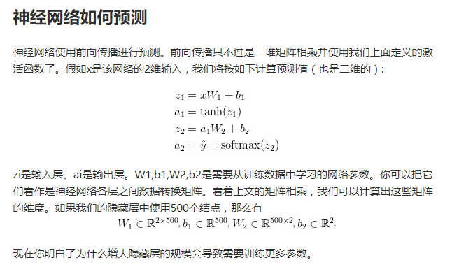
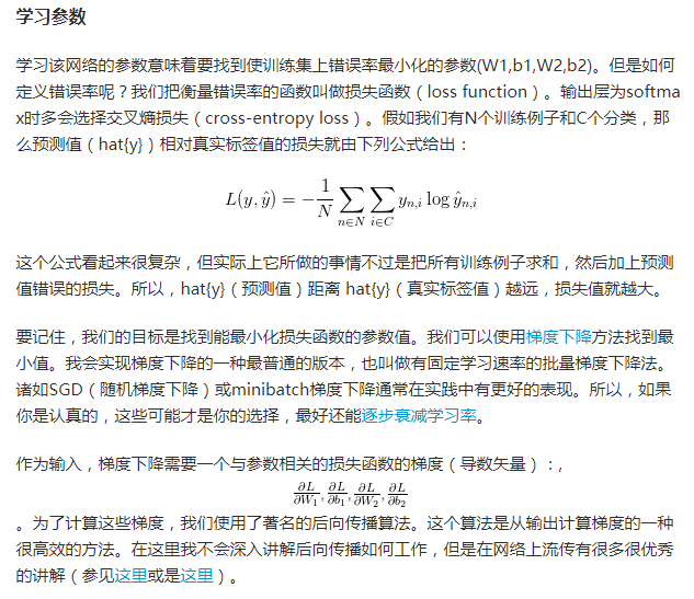
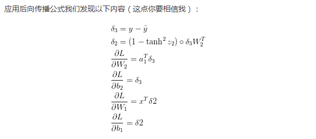
神经网络反射推到

https://www.cnblogs.com/biaoyu/archive/2015/06/20/4591304.html

交叉熵损失函数

http://blog.csdn.net/jasonzzj/article/details/52017438

三、实现思路

四、代码

 # %matplotlib inline   #add for display picture
 import numpy as np
 from sklearn import datasets
 from matplotlib import pyplot as plt
 # Generate a dataset and plot it
 np.random.seed(0)
 X, y = datasets.make_moons(200, noise=0.20)
 plt.scatter(X[:,0], X[:,1], s=40, c=y, cmap=plt.cm.Spectral)
 plt.show
 Out[24]:
 <function matplotlib.pyplot.show>

 In [19]:
 def plot_decision_boundary(pred_func):
     # Set min and max values and give it some padding
     x_min, x_max = X[:, 0].min() - .5, X[:, 0].max() + .5
     y_min, y_max = X[:, 1].min() - .5, X[:, 1].max() + .5
     h = 0.01
     # Generate a grid of points with distance h between them
     xx, yy = np.meshgrid(np.arange(x_min, x_max, h), np.arange(y_min, y_max, h))
     # Predict the function value for the whole gid
     Z = pred_func(np.c_[xx.ravel(), yy.ravel()])
     Z = Z.reshape(xx.shape)
     # Plot the contour and training examples
     plt.contourf(xx, yy, Z, cmap=plt.cm.Spectral)
     plt.scatter(X[:, 0], X[:, 1], c=y, cmap=plt.cm.Spectral)
 In [20]:
 from sklearn import linear_model
 # Train the logistic rgeression classifier
 clf = linear_model.LogisticRegressionCV()
 clf.fit(X, y)

 # Plot the decision boundary
 plot_decision_boundary(lambda x: clf.predict(x))
 plt.title("Logistic Regression")
 Out[20]:
 <matplotlib.text.Text at 0x1d21f527f98>

 In [14]:
 # Helper function to evaluate the total loss on the dataset
 def calculate_loss(model):
     W1, b1, W2, b2 = model['W1'], model['b1'], model['W2'], model['b2']
     # Forward propagation to calculate our predictions
     z1 = X.dot(W1) + b1
     a1 = np.tanh(z1)
     z2 = a1.dot(W2) + b2
     exp_scores = np.exp(z2)
     probs = exp_scores / np.sum(exp_scores, axis=1, keepdims=True)
     # Calculating the loss
     corect_logprobs = -np.log(probs[range(num_examples), y])
     data_loss = np.sum(corect_logprobs)
     # Add regulatization term to loss (optional)
     data_loss += reg_lambda/2 * (np.sum(np.square(W1)) + np.sum(np.square(W2)))
     return 1./num_examples * data_loss
 In [15]:
 # Helper function to predict an output (0 or 1)
 def predict(model, x):
     W1, b1, W2, b2 = model['W1'], model['b1'], model['W2'], model['b2']
     # Forward propagation
     z1 = x.dot(W1) + b1
     a1 = np.tanh(z1)
     z2 = a1.dot(W2) + b2
     exp_scores = np.exp(z2)
     probs = exp_scores / np.sum(exp_scores, axis=1, keepdims=True)
     return np.argmax(probs, axis=1)
 In [22]:
 # This function learns parameters for the neural network and returns the model.
 # - nn_hdim: Number of nodes in the hidden layer
 # - num_passes: Number of passes through the training data for gradient descent
 # - print_loss: If True, print the loss every 1000 iterations
 def build_model(nn_hdim, num_passes=20000, print_loss=False):

     # Initialize the parameters to random values. We need to learn these.
     np.random.seed(0)
     W1 = np.random.randn(nn_input_dim, nn_hdim) / np.sqrt(nn_input_dim)
     b1 = np.zeros((1, nn_hdim))
     W2 = np.random.randn(nn_hdim, nn_output_dim) / np.sqrt(nn_hdim)
     b2 = np.zeros((1, nn_output_dim))

     # This is what we return at the end
     model = {}

     # Gradient descent. For each batch...
     for i in range(0, num_passes):

         # Forward propagation
         z1 = X.dot(W1) + b1
         a1 = np.tanh(z1)
         z2 = a1.dot(W2) + b2
         exp_scores = np.exp(z2)
         probs = exp_scores / np.sum(exp_scores, axis=1, keepdims=True)

         # Backpropagation
         delta3 = probs
         delta3[range(num_examples), y] -= 1
         dW2 = (a1.T).dot(delta3)
         db2 = np.sum(delta3, axis=0, keepdims=True)
         delta2 = delta3.dot(W2.T) * (1 - np.power(a1, 2))
         dW1 = np.dot(X.T, delta2)
         db1 = np.sum(delta2, axis=0)

         # Add regularization terms (b1 and b2 don't have regularization terms)
         dW2 += reg_lambda * W2
         dW1 += reg_lambda * W1

         # Gradient descent parameter update
         W1 += -epsilon * dW1
         b1 += -epsilon * db1
         W2 += -epsilon * dW2
         b2 += -epsilon * db2

         # Assign new parameters to the model
         model = { 'W1': W1, 'b1': b1, 'W2': W2, 'b2': b2}

         # Optionally print the loss.
         # This is expensive because it uses the whole dataset, so we don't want to do it too often.
         if print_loss and i % 1000 == 0:
           print ("Loss after iteration %i: %f" %(i, calculate_loss(model)))

     return model
 In [17]:
 num_examples = len(X) # training set size
 nn_input_dim = 2 # input layer dimensionality
 nn_output_dim = 2 # output layer dimensionality

 # Gradient descent parameters (I picked these by hand)
 epsilon = 0.01 # learning rate for gradient descent
 reg_lambda = 0.01 # regularization strength
 In [23]:
 # Build a model with a 3-dimensional hidden layer
 model = build_model(3, print_loss=True)

 # Plot the decision boundary
 plot_decision_boundary(lambda x: predict(model, x))
 plt.title("Decision Boundary for hidden layer size 3")
 Loss after iteration 0: 0.432387
 Loss after iteration 1000: 0.068947
 Loss after iteration 2000: 0.068890
 Loss after iteration 3000: 0.071218
 Loss after iteration 4000: 0.071253
 Loss after iteration 5000: 0.071278
 Loss after iteration 6000: 0.071293
 Loss after iteration 7000: 0.071303
 Loss after iteration 8000: 0.071308
 Loss after iteration 9000: 0.071312
 Loss after iteration 10000: 0.071314
 Loss after iteration 11000: 0.071315
 Loss after iteration 12000: 0.071315
 Loss after iteration 13000: 0.071316
 Loss after iteration 14000: 0.071316
 Loss after iteration 15000: 0.071316
 Loss after iteration 16000: 0.071316
 Loss after iteration 17000: 0.071316
 Loss after iteration 18000: 0.071316
 Loss after iteration 19000: 0.071316
 Out[23]:
 <matplotlib.text.Text at 0x1d21f1fd8d0>

 In [ ]: