Handling Class Imbalance with R and Caret

When faced with classification tasks in the real world, it can be challenging to deal with an outcome where one class heavily outweighs the other (a.k.a., imbalanced classes). The following will be a two-part post on some of the techniques that can help to improve prediction performance in the case of imbalanced classes using R and caret. This first post provides a general overview of how these techniques can be implemented in practice, and the second post highlights some caveats to keep in mind when using these methods.

Evaluation metrics for classifiers

After building a classifier, you need to decide how to tell if it is doing a good job or not. Many evaluation metrics for classifiers exist, and can generally be divided into two main groups:

Threshold-dependent: This includes metrics like accuracy, precision, recall, and F1 score, which all require a confusion matrix to be calculated using a hard cutoff on predicted probabilities. These metrics are typically quite poor in the case of imbalanced classes, as statistical software inappropriately uses a default threshold of 0.50 resulting in the model predicting that all observations belong in the majority class.
Threshold-invariant: This includes metrics like area under the ROC curve (AUC), which quantifies true positive rate as a function of false positive rate for a variety of classification thresholds. Another way to interpret this metric is the probability that a random positive instance will have a higher estimated probability than a random negative instance.

Methods to improve performance on imbalanced data

A few of the more popular techniques to deal with class imbalance will be covered below, but the following list is nowhere near exhaustive. For brevity, a quick overview is provided. For a more substantial overview, I highly recommend this Silicon Valley Data Science blog post.

Class weights: impose a heavier cost when errors are made in the minority class
Down-sampling: randomly remove instances in the majority class
Up-sampling: randomly replicate instances in the minority class
Synthetic minority sampling technique (SMOTE): down samples the majority class and synthesizes new minority instances by interpolating between existing ones

It is important to note that these weighting and sampling techniques have the biggest impact on threshold-dependent metrics like accuracy, because they artificially move the threshold to be closer to what might be considered as the “optimal” location on a ROC curve. Threshold-invariant metrics can still be improved using these methods, but the effect will not be as pronounced.

Simulation set-up

To simulate class imbalance, the twoClassSim function from caret is used. Here, we simulate a separate training set and test set, each with 5000 observations. Additionally, we include 20 meaningful variables and 10 noise variables. The intercept argument controls the overall level of class imbalance and has been selected to yield a class imbalance of around 50:1.

library(dplyr) # for data manipulation

library(caret) # for model-building

library(DMwR) # for smote implementation

library(purrr) # for functional programming (map)

library(pROC) # for AUC calculations

set.seed(2969)

imbal_train <- twoClassSim(5000,

                           intercept = -25,

                           linearVars = 20,

                           noiseVars = 10)

imbal_test  <- twoClassSim(5000,

                           intercept = -25,

                           linearVars = 20,

                           noiseVars = 10)

prop.table(table(imbal_train$Class))

##

## Class1 Class2

## 0.9796 0.0204

Initial results

To model these data, a gradient boosting machine (gbm) is used as it can easily handle potential interactions and non-linearities that have been simulated above. Model hyperparameters are tuned using repeated cross-validation on the training set, repeating five times with ten folds used in each repeat. The AUC is used to evaluate the classifier to avoid having to make decisions about the classification threshold. Note that this code takes a little while to run due to the repeated cross-validation, so reduce the number of repeats to speed things up and/or use the verboseIter = TRUE argument in the trainControl function to keep track of the progress.

# Set up control function for training

ctrl <- trainControl(method = "repeatedcv",

                     number = 10,

                     repeats = 5,

                     summaryFunction = twoClassSummary,

                     classProbs = TRUE)

# Build a standard classifier using a gradient boosted machine

set.seed(5627)

orig_fit <- train(Class ~ .,

                  data = imbal_train,

                  method = "gbm",

                  verbose = FALSE,

                  metric = "ROC",

                  trControl = ctrl)

# Build custom AUC function to extract AUC

# from the caret model object

test_roc <- function(model, data) {

  roc(data$Class,

      predict(model, data, type = "prob")[, "Class2"])

}

orig_fit %>%

  test_roc(data = imbal_test) %>%

  auc()

## Area under the curve: 0.9575

Overall, the final model yields an AUC of 0.96 which is quite good. Can we improve it using the techniques outlined above?

Handling class imbalance with weighted or sampling methods

Both weighting and sampling methods are easy to employ in caret. Incorporating weights into the model can be handled by using the weights argument in thetrain function (assuming the model can handle weights in caret, see the listhere), while the sampling methods mentioned above can be implemented using the sampling argument in the trainControl function. Note that the same seeds were used for each model to ensure that results from the same cross-validation folds are being used.

Also keep in mind that for sampling methods, it is vital that you only sample the training set and not the test set as well. This means that when doing cross-validation, the sampling step must be done inside of the cross-validation procedure. Max Kuhn of the caret package gives a good overview of what happens when you don’t take this precaution in this caret documentation. Using the sampling argument in the trainControl function implements sampling correctly in the cross-validation procedure.

# Create model weights (they sum to one)

model_weights <- ifelse(imbal_train$Class == "Class1",

                        (1/table(imbal_train$Class)[1]) * 0.5,

                        (1/table(imbal_train$Class)[2]) * 0.5)

# Use the same seed to ensure same cross-validation splits

ctrl$seeds <- orig_fit$control$seeds

# Build weighted model

weighted_fit <- train(Class ~ .,

                      data = imbal_train,

                      method = "gbm",

                      verbose = FALSE,

                      weights = model_weights,

                      metric = "ROC",

                      trControl = ctrl)

# Build down-sampled model

ctrl$sampling <- "down"

down_fit <- train(Class ~ .,

                  data = imbal_train,

                  method = "gbm",

                  verbose = FALSE,

                  metric = "ROC",

                  trControl = ctrl)

# Build up-sampled model

ctrl$sampling <- "up"

up_fit <- train(Class ~ .,

                data = imbal_train,

                method = "gbm",

                verbose = FALSE,

                metric = "ROC",

                trControl = ctrl)

# Build smote model

ctrl$sampling <- "smote"

smote_fit <- train(Class ~ .,

                   data = imbal_train,

                   method = "gbm",

                   verbose = FALSE,

                   metric = "ROC",

                   trControl = ctrl)

Examining the AUC calculated on the test set shows a clear distinction between the original model implementation and those that incorporated either a weighting or sampling technique. The weighted method possessed the highest AUC value, followed by the sampling methods, with the original model implementation performing the worst.

# Examine results for test set

model_list <- list(original = orig_fit,

                   weighted = weighted_fit,

                   down = down_fit,

                   up = up_fit,

                   SMOTE = smote_fit)

model_list_roc <- model_list %>%

  map(test_roc, data = imbal_test)

model_list_roc %>%

  map(auc)

## $original

## Area under the curve: 0.9575

##

## $weighted

## Area under the curve: 0.9804

##

## $down

## Area under the curve: 0.9705

##

## $up

## Area under the curve: 0.9759

##

## $SMOTE

## Area under the curve: 0.976

We can examine the actual ROC curve to get a better idea of where the weighted and sampling models are outperforming the original model at a variety of classification thresholds. Here, we see that the weighted model seems to dominate the others throughout, while the original model lags between a false positive rate between 0% and 25%. This indicates that the other models have better early retrieval numbers. That is, the algorithm better identifies the true positives as a function of false positives for instances that are predicted as having a high probability of being in the minority class.

results_list_roc <- list(NA)

num_mod <- 1

for(the_roc in model_list_roc){

  results_list_roc[[num_mod]] <-

    data_frame(tpr = the_roc$sensitivities,

               fpr = 1 - the_roc$specificities,

               model = names(model_list)[num_mod])

  num_mod <- num_mod + 1

}

results_df_roc <- bind_rows(results_list_roc)

# Plot ROC curve for all 5 models

custom_col <- c("#000000", "#009E73", "#0072B2", "#D55E00", "#CC79A7")

ggplot(aes(x = fpr,  y = tpr, group = model), data = results_df_roc) +

  geom_line(aes(color = model), size = 1) +

  scale_color_manual(values = custom_col) +

  geom_abline(intercept = 0, slope = 1, color = "gray", size = 1) +

  theme_bw(base_size = 18)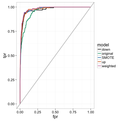

Final thoughts

In the above post, I outline some steps to help improve classification performance when you have imbalanced classes. Although weighting outperformed the sampling techniques in this simulation, this may not always be the case. Because of this, it is important to compare different techniques to see which works best for your data. I have actually found that in many cases, there is no huge benefit in using either weighting or sampling techniques when classes are moderately imbalanced (i.e., no worse than 10:1) in conjunction with a threshold-invariant metric like the AUC. In the next post, I will go over some caveats to keep in mind when using the AUC in the case of imbalanced classes and how other metrics can be more informative. Stay tuned!

转自：http://dpmartin42.github.io/blogposts/r/imbalanced-classes-part-1