
Spring 2017 Assignments2
一.作业要求
原版:http://cs231n.github.io/assignments2017/assignment2/
翻译:http://www.mooc.ai/course/268/learn?lessonid=2029#lesson/2029
二.作业收获及代码
完整代码地址:https://github.com/coldyan123/Assignment2
1 全连接网络
使用一种更模块化的方法,实现了线性层,Relu层,softmax层的前向和反向传播,然后使用for循环就可以实现任意层数的全连接Relu网络。并且还实现了sgd,带动量sgd,RMSProp,Adam几种优化方法和对比。这一部分很简单。
2 Batch Normalization
实现了BN层的前向传播和反向传播,关键代码为:
BN前向传播:
def batchnorm_forward(x, gamma, beta, bn_param):

    """

    Forward pass for batch normalization.

    During training the sample mean and (uncorrected) sample variance are

    computed from minibatch statistics and used to normalize the incoming data.

    During training we also keep an exponentially decaying running mean of the

    mean and variance of each feature, and these averages are used to normalize

    data at test-time.

    At each timestep we update the running averages for mean and variance using

    an exponential decay based on the momentum parameter:

    running_mean = momentum * running_mean + (1 - momentum) * sample_mean

    running_var = momentum * running_var + (1 - momentum) * sample_var

    Note that the batch normalization paper suggests a different test-time

    behavior: they compute sample mean and variance for each feature using a

    large number of training images rather than using a running average. For

    this implementation we have chosen to use running averages instead since

    they do not require an additional estimation step; the torch7

    implementation of batch normalization also uses running averages.

    Input:

    - x: Data of shape (N, D)

    - gamma: Scale parameter of shape (D,)

    - beta: Shift paremeter of shape (D,)

    - bn_param: Dictionary with the following keys:

      - mode: 'train' or 'test'; required

      - eps: Constant for numeric stability

      - momentum: Constant for running mean / variance.

      - running_mean: Array of shape (D,) giving running mean of features

      - running_var Array of shape (D,) giving running variance of features

    Returns a tuple of:

    - out: of shape (N, D)

    - cache: A tuple of values needed in the backward pass

    """

    mode = bn_param['mode']

    eps = bn_param.get('eps', 1e-5)

    momentum = bn_param.get('momentum', 0.9)

    N, D = x.shape

    running_mean = bn_param.get('running_mean', np.zeros(D, dtype=x.dtype))

    running_var = bn_param.get('running_var', np.zeros(D, dtype=x.dtype))

    out, cache = None, None

    if mode == 'train':

        #######################################################################

        # TODO: Implement the training-time forward pass for batch norm.      #

        # Use minibatch statistics to compute the mean and variance, use      #

        # these statistics to normalize the incoming data, and scale and      #

        # shift the normalized data using gamma and beta.                     #

        #                                                                     #

        # You should store the output in the variable out. Any intermediates  #

        # that you need for the backward pass should be stored in the cache   #

        # variable.                                                           #

        #                                                                     #

        # You should also use your computed sample mean and variance together #

        # with the momentum variable to update the running mean and running   #

        # variance, storing your result in the running_mean and running_var   #

        # variables.                                                          #

        #######################################################################

        sample_mean = np.mean(x, axis=0)

        sample_var = np.mean(x ** 2, axis=0) - sample_mean ** 2

        normal_x = (x - sample_mean) / np.sqrt(sample_var + eps)

        out = gamma * normal_x + beta

        running_mean = momentum * running_mean + (1 - momentum) * sample_mean

        running_var = momentum * running_var + (1 - momentum) * sample_var

        cache = (gamma, beta, sample_mean, sample_var, normal_x, eps, x)

        #######################################################################

        #                           END OF YOUR CODE                          #

        #######################################################################

    elif mode == 'test':

        #######################################################################

        # TODO: Implement the test-time forward pass for batch normalization. #

        # Use the running mean and variance to normalize the incoming data,   #

        # then scale and shift the normalized data using gamma and beta.      #

        # Store the result in the out variable.                               #

        #######################################################################

        normal_x = (x - running_mean) / np.sqrt(running_var + eps)

        out = gamma * normal_x + beta

        #######################################################################

        #                          END OF YOUR CODE                           #

        #######################################################################

    else:

        raise ValueError('Invalid forward batchnorm mode "%s"' % mode)

    # Store the updated running means back into bn_param

    bn_param['running_mean'] = running_mean

    bn_param['running_var'] = running_var

    return out, cache
BN反向传播(这里没有自己推,直接用的论文里的梯度公式):
def batchnorm_backward(dout, cache):

    """

    Backward pass for batch normalization.

    For this implementation, you should write out a computation graph for

    batch normalization on paper and propagate gradients backward through

    intermediate nodes.

    Inputs:

    - dout: Upstream derivatives, of shape (N, D)

    - cache: Variable of intermediates from batchnorm_forward.

    Returns a tuple of:

    - dx: Gradient with respect to inputs x, of shape (N, D)

    - dgamma: Gradient with respect to scale parameter gamma, of shape (D,)

    - dbeta: Gradient with respect to shift parameter beta, of shape (D,)

    """

    dx, dgamma, dbeta = None, None, None

    ###########################################################################

    # TODO: Implement the backward pass for batch normalization. Store the    #

    # results in the dx, dgamma, and dbeta variables.                         #

    ###########################################################################

    gamma, beta, sample_mean, sample_var, normal_x, eps, x = cache

    m = x.shape[0]

    dnormal_x = dout * gamma

    dvar = np.sum(dnormal_x * (x - sample_mean), axis=0) * (-0.5) * (sample_var + eps) ** (-1.5)

    dmean = np.sum(-1 / np.sqrt(sample_var + eps) * dnormal_x, axis=0) + dvar * np.sum(-2 * (x - sample_mean), axis=0) / m

    dx = 1 / np.sqrt(sample_var + eps) * dnormal_x + dvar * 2 * (x - sample_mean) / m + dmean / m

    dgamma = np.sum(dout * normal_x, axis=0)

    dbeta = np.sum(dout, axis=0)

    ###########################################################################

    #                             END OF YOUR CODE                            #

    ###########################################################################

    return dx, dgamma, dbeta
之后,将BN层加入到深度网络中进行实验:
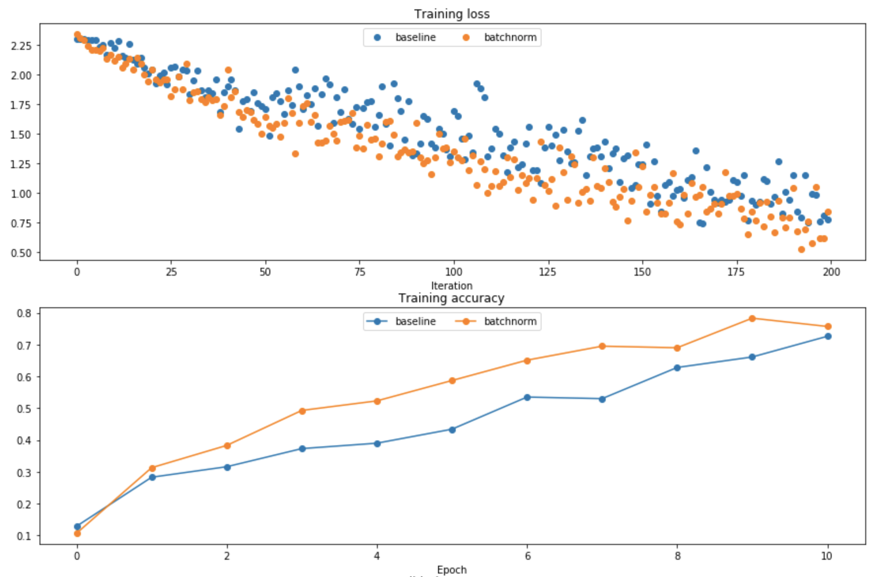
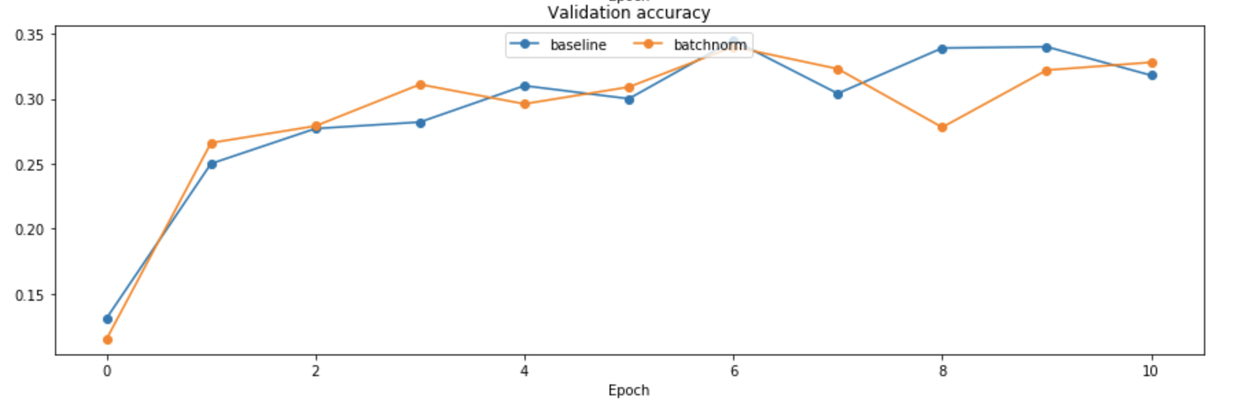
(1)实验1比较了使用和不使用BN的网络,发现使用BN之后收敛速度更快:
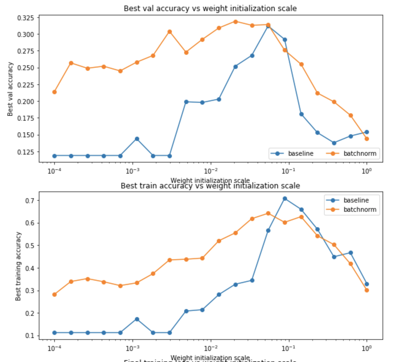
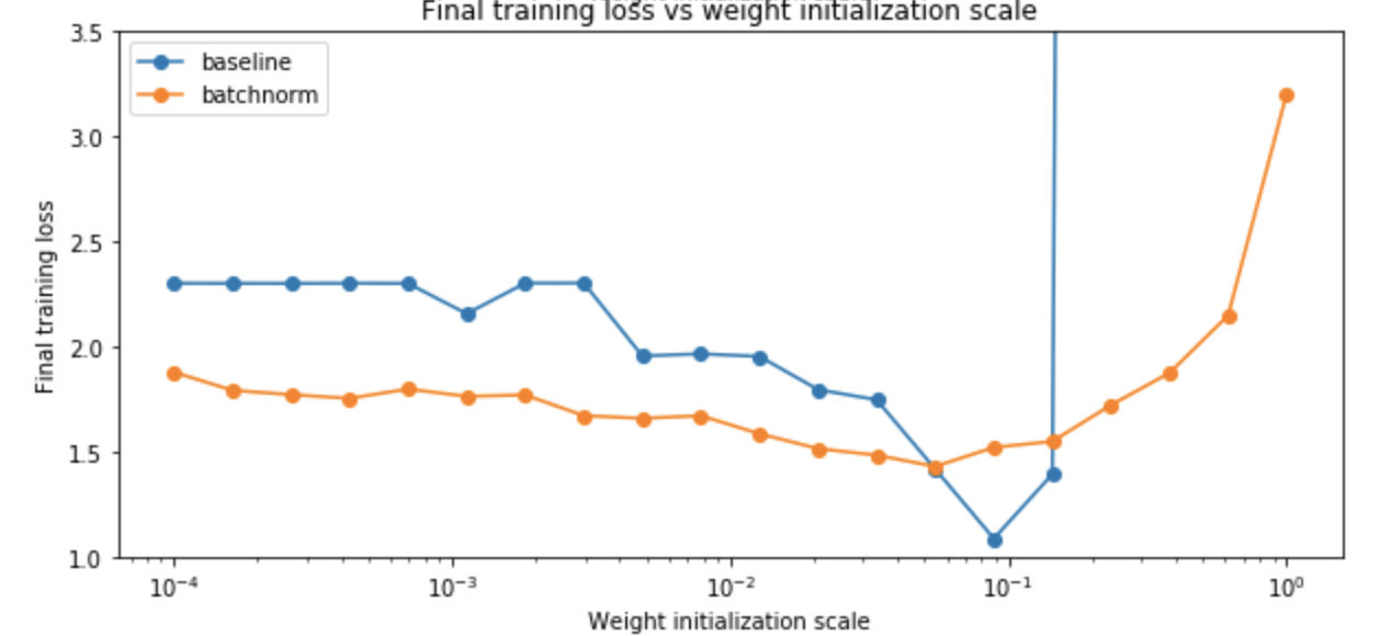
(2)实验2比较了使用和不使用BN的网络,初始化参数w对其性能的影响。发现使用BN的网络对初始化参数有更好的鲁棒性:
3 Dropout
(1)注意区别np.random.randn和np.random.rand,前者是生成服从标准正态分布的随机数,后者是生成0~1之间均匀分布的随机数。
(2)关键代码
Dropout层的前向传播:
if mode == 'train':

        mask = (np.random.rand(*x.shape) > p) / p

        out = x * mask

elif mode == 'test':

        out = x
注意这里实现的是inverted dropout,训练阶段通过dropout层乘以因子1/p,则测试阶段乘以p*1/p,刚好抵消,进而提高测试阶段的效率。
Dropout层的反向传播:
if mode == 'train':

        dx = dout * mask

 elif mode == 'test':

        dx = dout
(3)实验
实现了Dropout层的前向传播和反向传播,并加入到全连接网络中查看了正则化效果:

4 卷积神经网络
(1)一些numpy使用方法
①使用np.pad来做零填充。
②np.sum中,axis参数可以是元组,表示经过sum运算后,哪些维度将会消失掉。keepdims参数表示这些维度置为1,不消失。
③np.max中,与np.sum相同,axis参数表示哪些维度会消失掉。keepdims表示保持维度不消失,置为1。这些规则同样适用于np.mean,np.var等。
④特别要注意在进行整数语法切片后维度会丢失,导致广播出错。例如对一个(2,3)维的数组切片[1,:],生成的数组维度不是(1,3)而是(3,)
(2)灰度缩放和边缘检测
为了更好地理解卷积核,我们将滤波器分别设置为灰度缩放和边缘检测的形式:
# The first filter converts the image to grayscale.

# Set up the red, green, and blue channels of the filter.

w[0, 0, :, :] = [[0, 0, 0], [0, 0.0, 0], [0, 0, 0]]

w[0, 1, :, :] = [[0, 0, 0], [0, 0.0, 0], [0, 0, 0]]

w[0, 2, :, :] = [[0, 0, 0], [0, 1, 0], [0, 0, 0]]

# Second filter detects horizontal edges in the blue channel.

w[1, 2, :, :] = [[1, 2, 1], [0, 0, 0], [-1, -2, -1]]
这里的边缘检测卷积核又被称为Sobels算子,是计算机视觉中的一种边缘检测方法,详细介绍见https://en.wikipedia.org/wiki/Sobel_operator。我们通俗的理解一下Sobels算子为什么有边缘检测的效果:它的权重和为0,那么当滤波器探测到非边缘的时候(输入值在小窗口上变化不剧烈),输出约为0,当探测到边缘的时候(输入值在小窗口上变化剧烈),滤波器有大的输出。
最后的效果:

(3)卷积层的前向传播和反向传播(naive版)
前向传播:
def conv_forward_naive(x, w, b, conv_param):

    """

    A naive implementation of the forward pass for a convolutional layer.

    The input consists of N data points, each with C channels, height H and

    width W. We convolve each input with F different filters, where each filter

    spans all C channels and has height HH and width HH.

    Input:

    - x: Input data of shape (N, C, H, W)

    - w: Filter weights of shape (F, C, HH, WW)

    - b: Biases, of shape (F,)

    - conv_param: A dictionary with the following keys:

      - 'stride': The number of pixels between adjacent receptive fields in the

        horizontal and vertical directions.

      - 'pad': The number of pixels that will be used to zero-pad the input.

    Returns a tuple of:

    - out: Output data, of shape (N, F, H', W') where H' and W' are given by

      H' = 1 + (H + 2 * pad - HH) / stride

      W' = 1 + (W + 2 * pad - WW) / stride

    - cache: (x, w, b, conv_param)

    """

    out = None

    stride = conv_param['stride']

    pad = conv_param['pad']

    N, C, H, W = x.shape

    F, C, HH, WW = w.shape

    ###########################################################################

    # TODO: Implement the convolutional forward pass.                         #

    # Hint: you can use the function np.pad for padding.                      #

    ###########################################################################

    pad_x = np.pad(x, ((0, 0), (0, 0), (pad, pad), (pad, pad)), 'constant')

    H_out = int(1 + (H + 2 * pad - HH) / stride)

    W_out = int(1 + (W + 2 * pad - WW) / stride)

    out = np.zeros((N, F, H_out, W_out))

    for i in range(0, H_out):

        for j in range(0, W_out):

            x_part = pad_x[:, :, i * stride:i * stride + HH, j * stride:j * stride + WW]

            for k in range(0, F):

                out[:, k, i, j] = np.sum(x_part * w[k, :, :, :], axis=(1, 2, 3)) + b[k]

    ###########################################################################

    #                             END OF YOUR CODE                            #

    ###########################################################################

    cache = (x, w, b, conv_param)

    return out, cache
反向传播:
def conv_backward_naive(dout, cache):

    """

    A naive implementation of the backward pass for a convolutional layer.

    Inputs:

    - dout: Upstream derivatives.

    - cache: A tuple of (x, w, b, conv_param) as in conv_forward_naive

    Returns a tuple of:

    - dx: Gradient with respect to x

    - dw: Gradient with respect to w

    - db: Gradient with respect to b

    """

    dx, dw, db = None, None, None

    x, w, b, conv_param = cache

    stride = conv_param['stride']

    pad = conv_param['pad']

    H, W = (x.shape[2], x.shape[3])

    F, C, HH, WW = w.shape

    N, F, H_out, W_out = dout.shape

    ###########################################################################

    # TODO: Implement the convolutional backward pass.                        #

    ###########################################################################

    #cal db

    db = np.sum(dout, axis=(0, 2, 3))

    #cal dw

    dw = np.zeros(w.shape)

    pad_x = np.pad(x, ((0, 0), (0, 0), (pad, pad), (pad, pad)), 'constant')

    for i in range(0, H_out):

        for j in range(0, W_out):

            x_part = pad_x[:, :, i * stride:i * stride + HH, j * stride:j * stride + WW]

            for k in range(0, F):

                dw[k, :, :, :] += np.sum(x_part * dout[:, k, i, j].reshape(N, 1, 1, 1), axis=0)

    #cal dpad_x, dx

    dpad_x = np.zeros(pad_x.shape)

    for i in range(0, H_out):

        for j in range(0, W_out):

            dpad_x_part = dpad_x[:, :, i * stride:i * stride + HH, j * stride:j * stride + WW]

            for k in range(0, F):

                dpad_x_part += dout[:, k, i, j].reshape(N, 1, 1, 1) * w[k, :, :, :]

    dx = dpad_x[:, :, pad:pad+H, pad:pad+W]

    ###########################################################################

    #                             END OF YOUR CODE                            #

    ###########################################################################

    return dx, dw, db
卷积层的反向传播实现是一个难点,具体细节要好好琢磨代码,涉及到了大量的数组广播。实现的大体思路是:先考虑激活图中单个神经元的梯度是如何往回传的,然后遍历激活图,注意当不同路径的梯度传到同一个节点时,需要相加。
(4)max pooling层的前向传播和反向传播(naive版)
相比于卷积层,max pooling层很简单了。
前向传播:
def max_pool_forward_naive(x, pool_param):

    """

    A naive implementation of the forward pass for a max pooling layer.

    Inputs:

    - x: Input data, of shape (N, C, H, W)

    - pool_param: dictionary with the following keys:

      - 'pool_height': The height of each pooling region

      - 'pool_width': The width of each pooling region

      - 'stride': The distance between adjacent pooling regions

    Returns a tuple of:

    - out: Output data

    - cache: (x, pool_param)

    """

    out = None

    N, C, H, W = x.shape

    HH = pool_param['pool_height']

    WW = pool_param['pool_width']

    stride = pool_param['stride']

    ###########################################################################

    # TODO: Implement the max pooling forward pass                            #

    ###########################################################################

    H_out = int(1 + (H - HH) / stride)

    W_out = int(1 + (W - WW) / stride)

    out = np.zeros((N, C, H_out, W_out))

    for i in range(0, H_out):

        for j in range(0, W_out):

            x_part = x[:, :, i * stride:i * stride + HH, j * stride:j * stride + WW]

            out[:, :, i, j] = np.max(x_part, axis=(2, 3))

    ###########################################################################

    #                             END OF YOUR CODE                            #

    ###########################################################################

    cache = (x, pool_param)

    return out, cache
反向传播:
def max_pool_backward_naive(dout, cache):

    """

    A naive implementation of the backward pass for a max pooling layer.

    Inputs:

    - dout: Upstream derivatives

    - cache: A tuple of (x, pool_param) as in the forward pass.

    Returns:

    - dx: Gradient with respect to x

    """

    dx = None

    x, pool_param = cache

    N, C, H, W = x.shape

    HH = pool_param['pool_height']

    WW = pool_param['pool_width']

    stride = pool_param['stride']

    _, _, H_out, W_out = dout.shape

    ###########################################################################

    # TODO: Implement the max pooling backward pass                           #

    ###########################################################################

    dx = np.zeros(x.shape)

    for i in range(0, H_out):

        for j in range(0, W_out):

            dx_part = dx[:, :, i * stride:i * stride + HH, j * stride:j * stride + WW]

            x_part = x[:, :, i * stride:i * stride + HH, j * stride:j * stride + WW]

            dx_part += (np.max(x_part, axis=(2,3), keepdims=True) == x_part) * dout[:, :, i:i+1, j:j+1]

    ###########################################################################

    #                             END OF YOUR CODE                            #

    ###########################################################################

    return dx
(5) fast layer
作业中还给我们提供了卷积层和max pooling层的高效实现(不需要我们自己实现),这个实现基于Cython。
(6) 卷积网络中的Batch Normalization
卷积网络中,我们需要将处于同一个深度切面上的所有激活使用同样的方式标准化,因此需要在N*H*M上求均值和方差(标准的BN是在N上求均值方差),并且gamma和beta的大小为激活的深度C,即同一个深度切面使用同一个gamma和beta。对标准的Batch Normalization略做修改即可得到卷积网络中的Batch Normalization,称为空间Batch Normalization。实现如下:
前向传播:
def spatial_batchnorm_forward(x, gamma, beta, bn_param):

    """

    Computes the forward pass for spatial batch normalization.

    Inputs:

    - x: Input data of shape (N, C, H, W)

    - gamma: Scale parameter, of shape (C,)

    - beta: Shift parameter, of shape (C,)

    - bn_param: Dictionary with the following keys:

      - mode: 'train' or 'test'; required

      - eps: Constant for numeric stability

      - momentum: Constant for running mean / variance. momentum=0 means that

        old information is discarded completely at every time step, while

        momentum=1 means that new information is never incorporated. The

        default of momentum=0.9 should work well in most situations.

      - running_mean: Array of shape (D,) giving running mean of features

      - running_var Array of shape (D,) giving running variance of features

    Returns a tuple of:

    - out: Output data, of shape (N, C, H, W)

    - cache: Values needed for the backward pass

    """

    out, cache = None, None

    eps = bn_param.get('eps', 1e-5)

    momentum = bn_param.get('momentum', 0.9)

    C = x.shape[1]

    running_mean = bn_param.get('running_mean', np.zeros((1, C, 1, 1), dtype=x.dtype))

    running_var = bn_param.get('running_var', np.zeros((1, C, 1, 1), dtype=x.dtype))

    ###########################################################################

    # TODO: Implement the forward pass for spatial batch normalization.       #

    #                                                                         #

    # HINT: You can implement spatial batch normalization using the vanilla   #

    # version of batch normalization defined above. Your implementation should#

    # be very short; ours is less than five lines.                            #

    ###########################################################################

    if bn_param['mode'] == 'train':

        sample_mean = np.mean(x, axis=(0, 2, 3), keepdims=True)

        sample_var = np.var(x, axis=(0, 2, 3), keepdims=True)

        normal_x = (x - sample_mean) / np.sqrt(sample_var + eps)

        out = gamma.reshape(1, C, 1, 1) * normal_x + beta.reshape(1, C, 1, 1)

        running_mean = momentum * running_mean + (1 - momentum) * sample_mean

        running_var = momentum * running_var + (1 - momentum) * sample_var

        cache = (gamma, beta, sample_mean, sample_var, normal_x, eps, x)

    else:

        normal_x = (x - running_mean) / np.sqrt(running_var + eps)

        out = gamma.reshape(1, C, 1, 1) * normal_x + beta.reshape(1, C, 1, 1)

    ###########################################################################

    #                             END OF YOUR CODE                            #

    ###########################################################################

    bn_param['running_mean'] = running_mean

    bn_param['running_var'] = running_var

    return out, cache
反向传播:
def spatial_batchnorm_backward(dout, cache):

    """

    Computes the backward pass for spatial batch normalization.

    Inputs:

    - dout: Upstream derivatives, of shape (N, C, H, W)

    - cache: Values from the forward pass

    Returns a tuple of:

    - dx: Gradient with respect to inputs, of shape (N, C, H, W)

    - dgamma: Gradient with respect to scale parameter, of shape (C,)

    - dbeta: Gradient with respect to shift parameter, of shape (C,)

    """

    dx, dgamma, dbeta = None, None, None

    gamma, beta, sample_mean, sample_var, normal_x, eps, x = cache

    N, C, H, W = x.shape

    m = N * H * W

    C = dout.shape[1]

    ###########################################################################

    # TODO: Implement the backward pass for spatial batch normalization.      #

    #                                                                         #

    # HINT: You can implement spatial batch normalization using the vanilla   #

    # version of batch normalization defined above. Your implementation should#

    # be very short; ours is less than five lines.                            #

    ###########################################################################

    dnormal_x = dout * gamma.reshape(1, C, 1, 1)

    dvar = np.sum(dnormal_x * (x - sample_mean), axis=(0, 2, 3), keepdims=True) * (-0.5) * (sample_var + eps) ** (-1.5)

    dmean = np.sum(-1 / np.sqrt(sample_var + eps) * dnormal_x, axis=(0, 2, 3), keepdims=True) + dvar * np.sum(-2 * (x - sample_mean), axis=(0, 2, 3), keepdims=True) / m

    dx = 1 / np.sqrt(sample_var + eps) * dnormal_x + dvar * 2 * (x - sample_mean) / m + dmean / m

    dgamma = np.sum(dout * normal_x, axis=(0, 2, 3))

    dbeta = np.sum(dout, axis=(0, 2, 3))

    ###########################################################################

    #                             END OF YOUR CODE                            #

    ###########################################################################

    return dx, dgamma, dbeta
Spring 2017 Assignments2的更多相关文章
- cs231n spring 2017 lecture13 Generative Models 听课笔记
1. 非监督学习 监督学习有数据有标签,目的是学习数据和标签之间的映射关系.而无监督学习只有数据,没有标签,目的是学习数据额隐藏结构. 2. 生成模型(Generative Models) 已知训练数 ...
- cs231n spring 2017 lecture11 Detection and Segmentation 听课笔记
1. Semantic Segmentation 把每个像素分类到某个语义. 为了减少运算量,会先降采样再升采样.降采样一般用池化层,升采样有各种"Unpooling"." ...
- cs231n spring 2017 lecture9 CNN Architectures 听课笔记
参考<deeplearning.ai 卷积神经网络 Week 2 听课笔记>. 1. AlexNet(Krizhevsky et al. 2012),8层网络. 学会计算每一层的输出的sh ...
- cs231n spring 2017 lecture7 Training Neural Networks II 听课笔记
1. 优化: 1.1 随机梯度下降法(Stochasitc Gradient Decent, SGD)的问题: 1)对于condition number(Hessian矩阵最大和最小的奇异值的比值)很 ...
- cs231n spring 2017 lecture13 Generative Models
1. 非监督学习 监督学习有数据有标签,目的是学习数据和标签之间的映射关系.而无监督学习只有数据,没有标签,目的是学习数据额隐藏结构. 2. 生成模型(Generative Models) 已知训练数 ...
- cs231n spring 2017 lecture11 Detection and Segmentation
1. Semantic Segmentation 把每个像素分类到某个语义. 为了减少运算量,会先降采样再升采样.降采样一般用池化层,升采样有各种“Unpooling”.“Transpose Conv ...
- cs231n spring 2017 lecture9 CNN Architectures
参考<deeplearning.ai 卷积神经网络 Week 2 听课笔记>. 1. AlexNet(Krizhevsky et al. 2012),8层网络. 学会计算每一层的输出的sh ...
- cs231n spring 2017 lecture7 Training Neural Networks II
1. 优化: 1.1 随机梯度下降法(Stochasitc Gradient Decent, SGD)的问题: 1)对于condition number(Hessian矩阵最大和最小的奇异值的比值)很 ...
- cs231n spring 2017 lecture16 Adversarial Examples and Adversarial Training 听课笔记
(没太听明白,以后再听) 1. 如何欺骗神经网络? 这部分研究最开始是想探究神经网络到底是如何工作的.结果人们意外的发现,可以只改变原图一点点,人眼根本看不出变化,但是神经网络会给出完全不同的答案.比 ...
随机推荐
- Yii basic 模板支持连接多数据库
1.首先修改db配置文件,修改格式如下: return [ 'db' => [ 'class' => 'yii\db\Connection', 'dsn' => 'mysql:hos ...
- android_sdcard读写(三)
这次来个稍微复杂点的. package cn.com.sxp;import android.app.Activity;import android.app.ProgressDialog;import ...
- Sublime Text 3 实现C语言代码的编译和运行
Sublime Text 3 是一款优秀的代码编辑软件.界面简洁,轻巧快速,很受大家的欢迎. 最近开始用他来编辑数据结构的C语言代码,这就需要在新建编译系统.具体方法如下: 首先: 接下来是关键的一步 ...
- UVA11988 【Broken Keyboard (a.k.a. Beiju Text)】:题解
题目链接:https://www.luogu.org/problemnew/show/UVA11988 这题虽说是和链表有关的模拟,但其实并不是很需要啊,但蒟蒻用了(说的好听是练手,说的难听是太弱), ...
- Excel催化剂开源第13波-VSTO开发之DataGridView控件几个小坑
Excel催化剂内部大量使用了DataGridView,这其中有一些小坑,花了力气才解决的,在此给广大开发者作简单分享. 为何要使用DataGridView而不是其他控件如ListBox.ListVi ...
- npm常用命令(原创)
1.对于我们下载下来的node包,假设该包存在依赖情况执行: npm install(或者npm i) 下载依赖包: 下载依赖成功过后,文件夹内会产生package-lock.json文件: 2.下载 ...
- IDEA自定义配置
目录 1 常规设置 1 修改字体大小 2 创建文件时 增加注释信息 3 项目编码为UTF-8 4 properties 文件编码为UTF-8且Transparent native-to-ascii c ...
- 【iOS】Error: Error Domain=PBErrorDomain Code=7 "Cannot connect to pasteboard server
这几天在用 Swift 开发一个简单的键盘扩展,真机调试时遇到了这个问题,详细信息如下: ***[:] Could not save pasteboard named com.apple.UIKit. ...
- 【iOS】Masonry 自动布局 MASViewConstraint.m:207 错误
问题详情: Assertion failure 报错原因: make.right.equalTo([_imageView superview]).right.with.offset(-); make. ...
- Code blocks返回错误代码:Process returned -1073741819 (0xC0000005)
循环语句访问链表时,返回了错误代码: 逐项排查后,发现是由while循环引起的: 附上出错代码: do{ L=L->post; printf("%05d %d %05d\n" ...