（转）GANs and Divergence Minimization

GANs and Divergence Minimization

2018-12-22 09:38:27

 

 

This blog is copied from: https://colinraffel.com/blog/gans-and-divergence-minimization.html 

 

 

This post discusses a perspective on GANs which is not new but I think is often overlooked. I'll use this perspective to motivate an evaluation procedure for GANs which I think is underutilized and understudied. For setup, I'll first give a quick review of maximum likelihood estimation and the forward KL divergence; if you're familiar with these concepts you can skip to section 3.

The Forward KL divergence and Maximum Likelihood

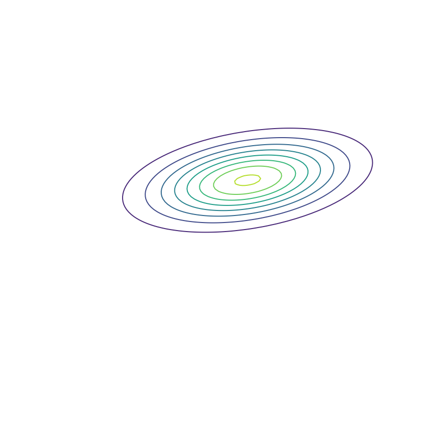
In generative modeling, our goal is to produce a model qθ(x)qθ(x) of some “true” underlying probability distribution p(x)p(x). For the moment, let's consider modeling the 2D Gaussian distribution shown below. This is a toy example; in practice we want to model extremely complex distributions in high dimensions, such as the distribution of natural images.

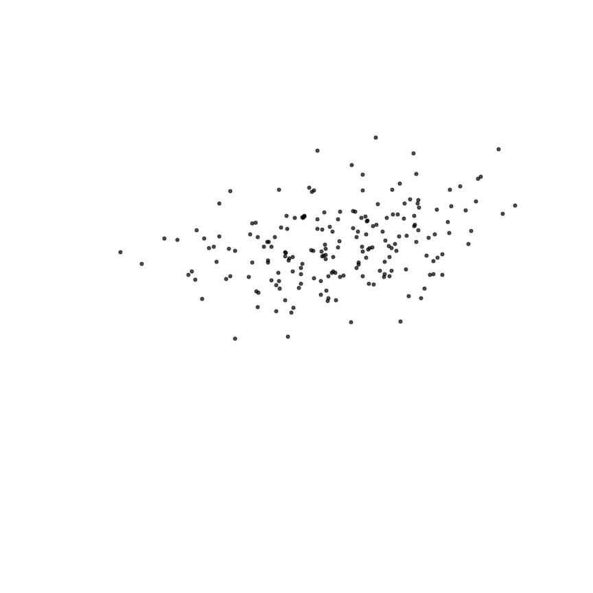
We don't actually have access to the true distribution; instead, we have access to samples drawn as x∼px∼p. Shown below are some samples from this Gaussian distribution. We want to be able to choose the parameters of our model qθ(x)qθ(x) using these samples alone.

Let's fit a Gaussian distribution to these samples. This will produce our model qθ(x)qθ(x), which ideally will match the true distribution p(x)p(x). To do so, we need to adjust the parameters θθ (in this case, the mean and covariance) of our Gaussian model so that they minimize some measure of the difference between qθ(x)qθ(x) and the samples from p(x)p(x). In practice, we'll use gradient descent over θθ for this minimization. Let's start by using the KL divergence as a measure of the difference. Our goal will be to minimize the KL divergence (using gradient descent) between p(x)p(x) and qθ(x)qθ(x) to find the best set of parameters θ∗θ∗:

θ∗===argminθKL(p(x)||qθ(x))argminθEx∼p[logp(x)−logqθ(x)]argminθEx∼p[logp(x)]−Ex∼p[logqθ(x)](1)(2)(3)(1)θ∗=argminθKL(p(x)||qθ(x))(2)=argminθEx∼p[log⁡p(x)−log⁡qθ(x)](3)=argminθEx∼p[log⁡p(x)]−Ex∼p[log⁡qθ(x)]

where the separation of terms in eqn. 33 comes from the linearity of expectation. The first term, Ex∼p[logp(x)]Ex∼p[log⁡p(x)], is just the negative entropy of the true distribution p(x)p(x). Changing θθ won't change this quantity, so we can ignore it for the purposes of finding θ∗θ∗. This is nice because we also can't compute it in practice — it requires evaluating p(x)p(x), and we do not have access to the true distribution. This gives us

θ∗===argminθEx∼p[logp(x)]−Ex∼p[logqθ(x)]argminθ−Ex∼p[logqθ(x)]argmaxθEx∼p[logqθ(x)](4)(5)(6)(4)θ∗=argminθEx∼p[log⁡p(x)]−Ex∼p[log⁡qθ(x)](5)=argminθ−Ex∼p[log⁡qθ(x)](6)=argmaxθEx∼p[log⁡qθ(x)]

Eqn. 66 states that we want to find the value of θθ which assigns samples from p(x)p(x) the highest possible log probability under qθ(x)qθ(x). This is exactly the equation for maximum likelihood estimation, which we have shown is equivalent to minimizing KL(p(x)||qθ(x))KL(p(x)||qθ(x)). Let's see what happens when we optimize the parameters θθ of our Gaussian qθ(x)qθ(x) to fit the samples from p(x)p(x)via maximum likelihood:

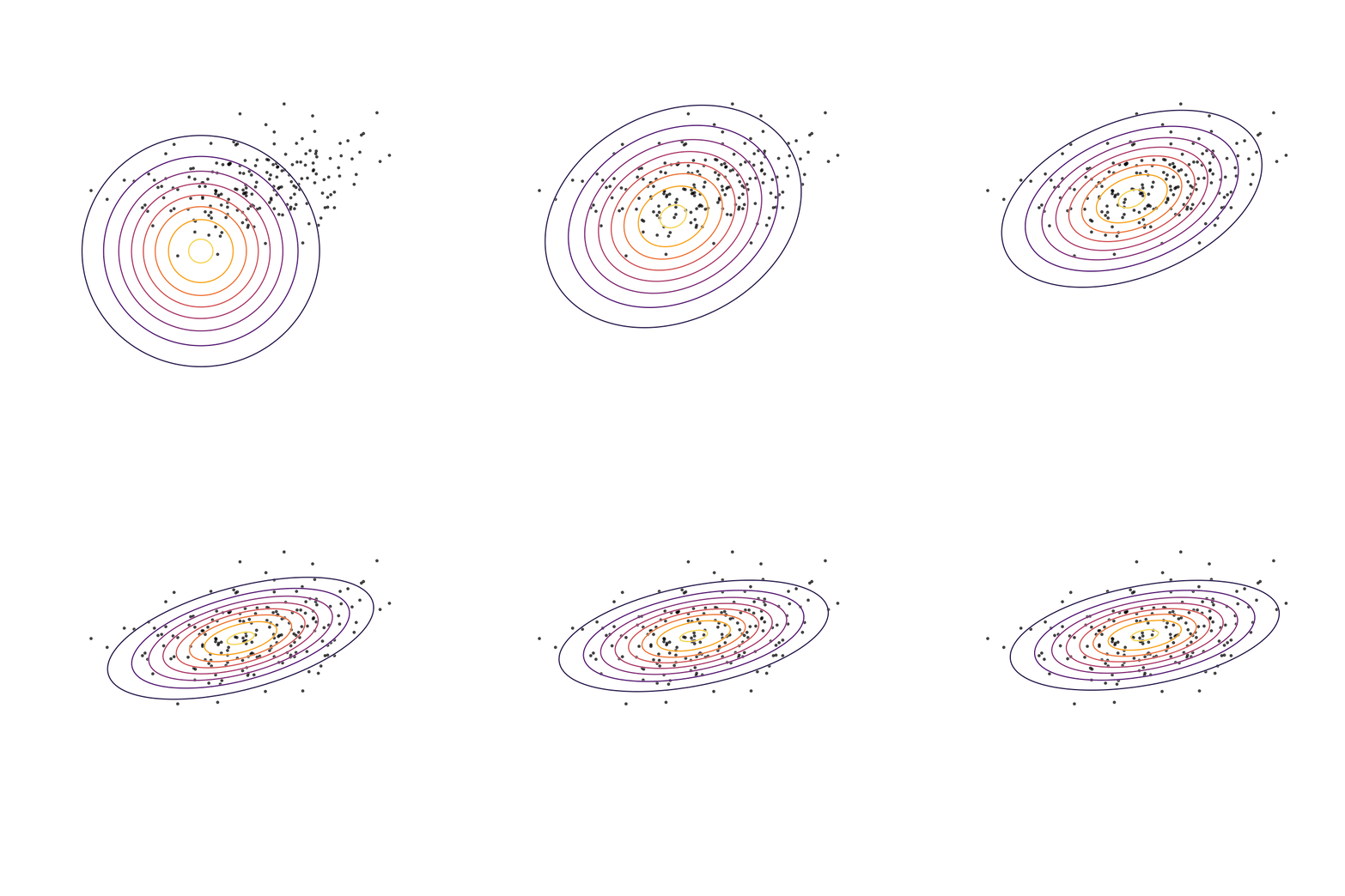
Looks like a good fit!

Model Misspecification

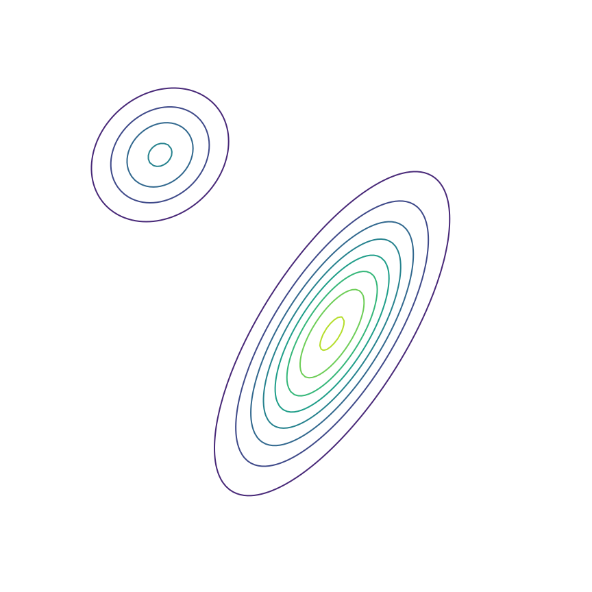
The above example was somewhat unrealistic in the sense that both our true distribution p(x)p(x)and our model qθ(x)qθ(x) were Gaussian distributions. To make things a bit harder, let's consider the case where our true distribution is a mixture of Gaussians:

Here's what happens when we fit a 2D Gaussian distribution to samples from this mixture of Gaussians using maximum likelihood:

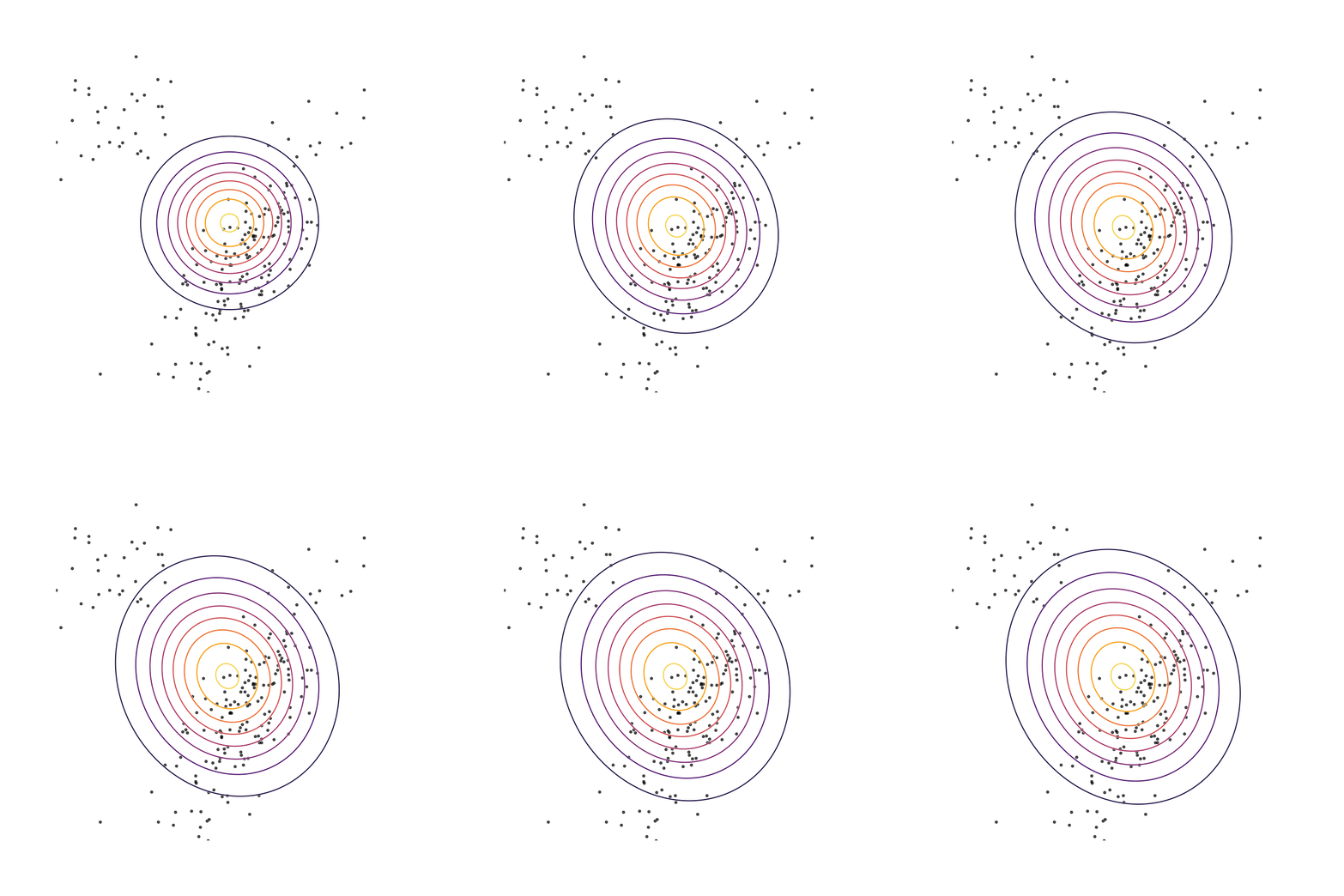
We can see that qθ(x)qθ(x) “spreads out” to try to cover the entirety of p(x)p(x). Why does this happen? Let's look at the maximum likelihood equation again:

θ∗=argmaxθEx∼p[logqθ(x)](7)(7)θ∗=argmaxθEx∼p[log⁡qθ(x)]

What happens if we draw a sample from p(x)p(x) and it has low probability under qθ(x)qθ(x)? As qθ(x)qθ(x)approaches zero for some x∼px∼p, logqθ(x)log⁡qθ(x) goes to negative infinity. Since we are trying to maximize qθ(x)qθ(x), this means it's really really bad if we draw a sample from p(x)p(x) and qθ(x)qθ(x)assigns a low probability to it. In contrast, if some xx has low probability under p(x)p(x) but high probability under qθ(x)qθ(x), this will not affect maximum likelihood loss much. The result is that the estimated model tries to cover the entire support of the true distribution, and in doing so ends up assigning probability mass to regions of space (between the two mixture components) which have low probability under p(x)p(x). In looser terms, this means that samples from qθ(x)qθ(x)might be “unrealistic”.

The Reverse KL Divergence

To get around this issue, let's try something simple: Instead of minimizing the KL divergence between p(x)p(x) and qθ(x)qθ(x), let's try minimizing the KL divergence between qθ(x)qθ(x) and p(x)p(x). This is called the “reverse” KL divergence:

θ∗====argminθKL(qθ||p)argminθEx∼qθ[logqθ(x)−logp(x)]argminθEx∼qθ[logqθ(x)]−Ex∼qθ[logp(x)]argmaxθ−Ex∼qθ[logqθ(x)]+Ex∼qθ[logp(x)](8)(9)(10)(11)(8)θ∗=argminθKL(qθ||p)(9)=argminθEx∼qθ[log⁡qθ(x)−log⁡p(x)](10)=argminθEx∼qθ[log⁡qθ(x)]−Ex∼qθ[log⁡p(x)](11)=argmaxθ−Ex∼qθ[log⁡qθ(x)]+Ex∼qθ[log⁡p(x)]

The two terms in equation 1111 each have an intuitive description: The first term −Ex∼qθ[logqθ(x)]−Ex∼qθ[log⁡qθ(x)] is simply the entropy of qθ(x)qθ(x). So, we want our model to have high entropy, or to put it intuitively, its probability mass should be as spread out as possible. The second term Ex∼qθ[logp(x)]Ex∼qθ[log⁡p(x)] is the log probability of samples from qθ(x)qθ(x) under the true distribution p(x)p(x). In other words, any sample from qθ(x)qθ(x) has to be reasonably “realistic” according to our true distribution. Note that without the first term, our model could “cheat” by simply assigning all of its probability mass to a single sample which has high probability under p(x)p(x). This solution is essentially memorization of a single point, and the entropy term discourages this behavior. Let's see what happens when we fit a 2D Gaussian to the mixture of Gaussians using the reverse KL divergence:

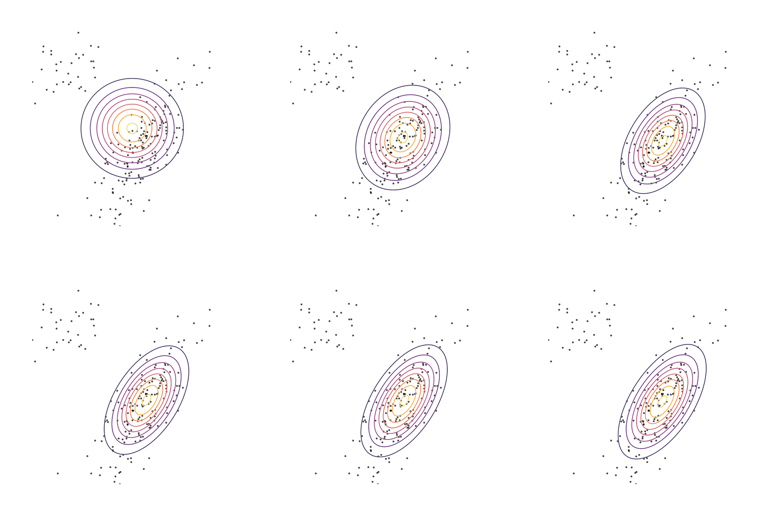
Our model basically picks a single mode and models it well. This solution is reasonably high-entropy, and any sample from the estimated distribution has a reasonably high probability under p(x)p(x), because the support of qθqθ is basically a subset of the support of p(x)p(x). The drawback here is that we are basically missing an entire mixture component of the true distribution.

When might this be a desirable solution? As an example, let's consider image superresolution, where we want to recover a high-resolution image (right) from a low-resolution version (left):

This figure was made by my colleague David Berthelot. In this task, there are multiple possible “good” solutions. In this case, it may be much more important that our model produces a single high-quality output than that it correctly models the distribution over all possible outputs. Of course, reverse KL provides no control over which output is chosen, just that the distribution learned by the model has high probability under the true distribution. In contrast, maximum likelihood can result in a “worse” solution in practice because it might produce low-quality or incorrect outputs by virtue of trying to model every possible outcome despite model misspecification or insufficient capacity. Note that one way to deal with this is to train a model with more capacity; a recent example of this approach is Glow [kingma2018], a maximum likelihood-based model which achieves impressive results with over 100 million parameters.

Generative Adversarial Networks

In using the reverse KL divergence above, I've glossed over an important detail: We can't actually compute the second term Ex∼qθ[logp(x)]Ex∼qθ[log⁡p(x)] because it requires evaluating the true probability p(x)p(x) of a sample x∼qθx∼qθ. In practice, we don't have access to the true distribution, we only have access to samples from it. So, we can't actually use reverse KL divergence to optimize the parameters of our model. In Section 3, I “cheated” since I knew what the true model was in our toy problem.

So far, we have been fitting the parameters of qθ(x)qθ(x) by minimizing a divergence between qθ(x)qθ(x)and p(x)p(x) — the forward KL divergence in Section 1 and the reverse KL divergence in Section 3. Generative Adversarial Networks (GANs) [goodfellow2014] fit the parameters of qθ(x)qθ(x) via the following objective:

θ∗=argminθmaxϕEx∼p,x^∼qθV(fϕ(x),fϕ(x^))(12)(12)θ∗=argminθmaxϕEx∼p,x^∼qθV(fϕ(x),fϕ(x^))

The first bit of this equation is unchanged: We are still choosing θ∗θ∗ via a minimization over θθ. What has changed is the quantity we're minimizing. Instead of minimizing over some analytically defined divergence, we're minimizing the quantity maxϕEx∼p,x^∼qθV(fϕ(x),fϕ(x^))maxϕEx∼p,x^∼qθV(fϕ(x),fϕ(x^))which can be loosely considered a “learned divergence”. Let's unpack this a bit: fϕ(x)fϕ(x) is a neural network typically called the “discriminator” or “critic” and is parametrized by ϕϕ. It takes in samples from p(x)p(x) or qθ(x)qθ(x) and outputs a scalar value. V(⋅,⋅)V(⋅,⋅) is a loss function which fϕ(x)fϕ(x) is trained to maximize. The original GAN paper used the following loss function:

V(fϕ(x),fϕ(x^))=logfϕ(x)+log[1−fϕ(x^)](13)(13)V(fϕ(x),fϕ(x^))=log⁡fϕ(x)+log⁡[1−fϕ(x^)]

where fϕ(x)fϕ(x) is required to output a value between 0 and 1.

Interestingly, if fϕ(x)fϕ(x) can represent any function, choosing θ∗θ∗ via Equation 1212 using the loss function in Equation 1313 is equivalent to minimizing the Jensen-Shannon divergence between p(x)p(x) and qθ(x)qθ(x). More generally, it is possible to construct loss functions V(⋅,⋅)V(⋅,⋅) and critic architectures which result (in some limit) in minimization of some analytical divergence. This can allow for minimization of divergences which are otherwise intractable or impossible to minimize directly. For example, [nowozin2016] showed that the following loss function corresponds to minimization of the reverse KL divergence:

V(fϕ(x),fϕ(x^))=−exp(fϕ(x))+1+fϕ(x^)(14)(14)V(fϕ(x),fϕ(x^))=−exp⁡(fϕ(x))+1+fϕ(x^)

Let's go ahead and do this in the example above of fitting a 2D Gaussian to a mixture of Gaussians:

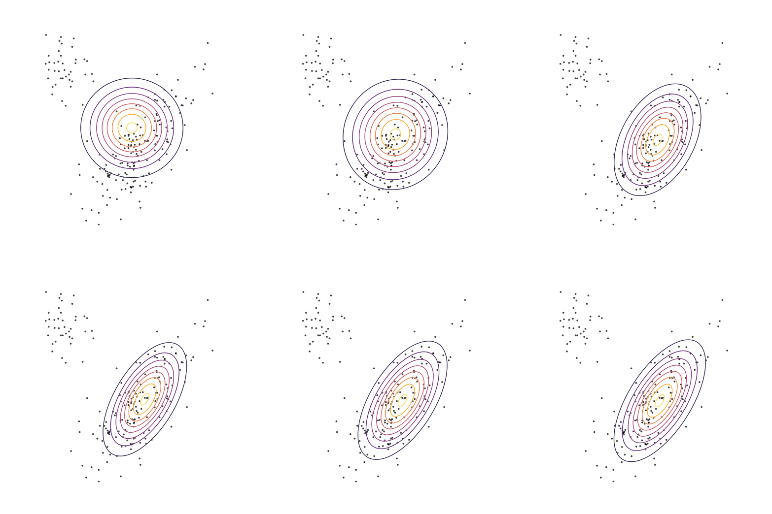
Sure enough, the solution found by minimizing the GAN objective with the loss function in Equation 1414 looks roughly the same as the one found by minimizing the reverse KL divergence, but did not require “cheating” by evaluating p(x)p(x).

To re-emphasize the importance of this, the GAN framework opens up the possibility of minimizing divergences which we can't compute or minimize otherwise. This allows learning generative models using objectives other than maximum likelihood, which has been the dominant paradigm for roughly a century. Maximum likelihood's ubiquity is not without good reason — it is tractable (unlike, say, the reverse KL divergence) and has nice theoretical properties, like its efficiency and consistency. Nevertheless, the GAN framework opens the possibility of using alternative objectives which, for example and loosely speaking, prioritize “realism” over covering the entire support of p(x)p(x).

As a final note on this perspective, the statements above about how GANs minimize some underlying analytical divergence can lead people thinking of them as “just minimizing the Jensen-Shannon (or whichever other) divergence”. However, the proofs of these statements rely on assumptions that don't hold up in practice. For example, we don't expect fϕ(x)fϕ(x) to have the ability to represent any function for any reasonable neural network architecture. Further, we perform the maximization over ϕϕ via gradient ascent, which for neural networks is not guaranteed to converge to any kind of optimal solution. As a result, stating that GANs are simply minimizing some analytical divergence is misleading. To me, this is actually another thing that makes GANs interesting, because it allows us to imbue prior knowledge about our problem in our “learned divergence”. For example, if we use a convolutional neural network for fϕ(x)fϕ(x), this suggests some amount of translation invariance in the objective minimized by qθ(x)qθ(x), which might be a useful structural prior for modeling the distribution of natural images.

Evaluation

One appealing characteristic of maximum likelihood estimation is that it facilitates a natural measure of “generalization”: Assuming that we hold out a set of samples from p(x)p(x) which were not used to train qθ(x)qθ(x) (call this set xtestxtest), we can compute the likelihood assigned by our model to these samples:

Ex∼p[logqθ(x)]≈1|xtest|∑x∈xtestlogqθ(x)(15)(15)Ex∼p[log⁡qθ(x)]≈1|xtest|∑x∈xtestlog⁡qθ(x)

If our model assigns a similar likelihood to these samples as it did to those it was trained on, this suggests that it has not “overfit”. Note that Equation 1515 simply computes the divergence used to train the model (ignoring the data entropy term, which is independent of the model) over xtestxtest.

Typically, the GAN framework is not thought to allow this kind of evaluation. As a result, various ad-hoc and task-specific evaluation functions have been proposed (such as the Inception Score and the Frechet Inception Distance for modeling natural images). However, following the reasoning above actually provides a natural analog to the evaluation procedure used for maximum likelihood: After training our model, we train an “independent critic” (used only for evaluation) from scratch on our held-out set of samples from p(x)p(x) and samples from qθ(x)qθ(x) with θθ held fixed:

maxϕEx∼p,x^∼qθV(fϕ(x),fϕ(x^))≈maxϕ1|xtest|∑x∈xtestEx^∼qθV(fϕ(x),fϕ(x^))(16)(16)maxϕEx∼p,x^∼qθV(fϕ(x),fϕ(x^))≈maxϕ1|xtest|∑x∈xtestEx^∼qθV(fϕ(x),fϕ(x^))

Both Equation 1515 and Equation 1616 compute the divergence used for training our model over the samples in xtestxtest. Of course, Equation 1616 requires training a neural network from scratch, but it nevertheless loosely represents the divergence we used to find the parameters θθ.

While not widely used, this evaluation procedure has seen some study, for example in [danihelka2017] and [im2018]. In recent work [gulrajani2018], we argue that this evaluation procedure facilitates some notion of generalization and include some experiments to gain better insight into its behavior. I plan to discuss this work in a future blog post.

Pointers

The perspective given in this blog post is not new. [theis2015] and [huszar2015] both discuss the different behavior of maximum likelihood, reverse KL, and GAN-based training in terms of support coverage. Huszár also has a few follow-up blog posts on the subject [huszar2016a], [huszar2016b]. [poole2016] further develops the use of the GAN framework for minimizing arbitrary f-divergences. [fedus2017] demonstrates how GANs are not always minimizing some analytical divergence in practice. [huang2017] provides some perspective on the idea that the design of the critic architecture allows us to imbue task-specific priors in our objective. Finally, [arora2017] and [liu2017] provide some theory about the “adversarial divergences” learned and optimized in the GAN framework.

Acknowledgements

Thanks to Ben Poole, Durk Kingma, Avital Oliver, and Anselm Levskaya for their feedback on this blog post.

References

[goodfellow2014] Ian Goodfellow, Jean Pouget-Abadie, Mehdi Mirza, Bing Xu, David Warde-Farley, Sherjil Ozair, Aaron Courville, and Yoshua Bengio. Generative Adversarial Networks. arXiv:1406.2661, 2014.

[nowozin2016] Sebastian Nowozin, Botond Cseke, and Ryota Tomioka. f-GAN: Training Generative Neural Samplers using Variational Divergence Minimization. arXiv:1606.00709, 2016.

[danihelka2017] Ivo Danihelka, Balaji Lakshminarayanan, Benigno Uria, Daan Wierstra, and Peter Dayan. Comparison of Maximum Likelihood and GAN-based training of Real NVPs. arXiv:1705.05263, 2017.

[im2018] Daniel Jiwoong Im, He Ma, Graham Taylor, and Kristin Branson. Quantitatively Evaluating GANs With Divergences Proposed for Training. arXiv:1803.01045, 2018.

[gulrajani2018] Ishaan Gulrajani, Colin Raffel, and Luke Metz. Towards GAN Benchmarks Which Require Generalization. To appear at ICLR 2019.

[theis2015] Lucas Theis, Aäron van den Oord, and Matthias Bethge. A note on the evaluation of generative models. arXiv:1511.01844, 2015.

[huszar2015] Ferenc Huszár. How (not) to Train your Generative Model: Scheduled Sampling, Likelihood, Adversary? arXiv:1511.05101, 2015.

[huszar2016a] Ferenc Huszár. An Alternative Update Rule for Generative Adversarial Networks. https://www.inference.vc/an-alternative-update-rule-for-generative-adversarial-networks/, 2015.

[huszar2016b] Ferenc Huszár. Understanding Minibatch Discrimination in GANs. https://www.inference.vc/understanding-minibatch-discrimination-in-gans/, 2015.

[poole2016] Ben Poole, Alexander A. Alemi, Jascha Sohl-Dickstein, and Anelia Angelova. Improved generator objectives for GANs. arXiv:1612.02780, 2016.

[fedus2017] William Fedus, Mihaela Rosca, Balaji Lakshminarayanan, Andrew M. Dai, Shakir Mohamed, and Ian Goodfellow. Many Paths to Equilibrium: GANs Do Not Need to Decrease a Divergence At Every Step. arXiv:1710.08446, 2017.

[huang2017] Gabriel Huang, Hugo Berard, Ahmed Touati, Gauthier Gidel, Pascal Vincent, and Simon Lacoste-Julien. Parametric Adversarial Divergences are Good Task Losses for Generative Modeling. arXiv:1708.02511, 2017.

[arora2017] Sanjeev Arora, Rong Ge, Yingyu Liang, Tengyu Ma, and Yi Zhang. Generalization and Equilibrium in Generative Adversarial Nets (GANs). arXiv:1703.00573, 2017.

[liu2017] Shuang Liu, Olivier Bousquet, and Kamalika Chaudhuri. Approximation and Convergence Properties of Generative Adversarial Learning. arXiv:1705.08991, 2017.