Lucas–Kanade光流算法学习

Lucas–Kanade光流算法是一种两帧差分的光流估计算法。它由Bruce D. Lucas 和 Takeo Kanade提出。

        光流(Optical flow or optic flow)是一种运动模式，这种运动模式指的是一个物体、表面、边缘在一个视角下由一个观察者（比如眼睛、摄像头等）和背景之间形成的明显移动。光流技术，如运动检测和图像分割，时间碰撞，运动补偿编码，三维立体视差，都是利用了这种边缘或表面运动的技术。

      有序的图像可以估计出二维图像的瞬时图像速率或离散图像转移。

光流算法评估了两幅图像的之间的变形，它的基本假设是体素和图像像素守恒。它假设一个物体的颜色在前后两帧没有巨大而明显的变化。基于这个思路，我们可以得到图像约束方程。不同的光流算法解决了假定了不同附加条件的光流问题。

Lucas–Kanade算法：
这个算法是最常见，最流行的。它计算两帧在时间t 到t + δt之间每个每个像素点位置的移动。 由于它是基于图像信号的泰勒级数，这种方法称为差分，这就是对于空间和时间坐标使用偏导数。
图像约束方程可以写为I (x ,y ,z ,t ) = I (x + δx ,y + δy ,z + δz ,t + δt )
I(x, y,z, t) 为在（x,y,z）位置的体素。
我们假设移动足够的小，那么对图像约束方程使用泰勒公式，我们可以得到：

H.O.T. 指更高阶，在移动足够小的情况下可以忽略。从这个方程中我们可以得到：

或者

我们得到：

V _x ,V _y ,V _z 分别是I(x,y,z,t)的光流向量中x，y，z的组成。 , , 和 则是图像在(x ,y ,z ,t )这一点向相应方向的差分 。
所以

I _x V _x + I _y V _y + I _z V _z = − I _t。

写做：

这个方程有三个未知量，尚不能被解决，这也就是所谓光流算法的光圈问题。那么要找到光流向量则需要另一套解决的方案。而Lucas-Kanade算法是一个非迭代的算法：

假设流(Vx,Vy,Vz)在一个大小为m*m*m(m>1)的小窗中是一个常数，那么从像素1...n , n = m ³ 中可以得到下列一组方程：（也就是说，对于这多个点，它们三个方向的速度是一样的）即，假设了在一个像素的周围的一个小的窗口内的所有像素点的光流大小是相同的。

（

而两帧图像之间的变化，就是t方向的梯度值，可以理解为当前像素点沿着光流方向运动而得到的，所以我们可以得到上边的这个式子。令：

）

三个未知数但是有多于三个的方程，这个方程组自然是个超定方程，也就是说方程组内有冗余，方程组可以表示为：

记作：

为了解决这个超定问题，我们采用最小二乘法：

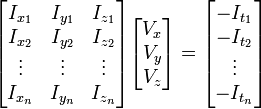
or

得到：

其中的求和是从1到n。

这也就是说寻找光流可以通过在四维上图像导数的分别累加得出。我们还需要一个权重函数W(i, j,k) ， 来突出窗口中心点的坐标。高斯函数做这项工作是非常合适的，

这个算法的不足在于它不能产生一个密度很高的流向量，例如在运动的边缘和黑大的同质区域中的微小移动方面流信息会很快的褪去。它的优点在于有噪声存在的鲁棒性还是可以的。

补充：opencv里实现的看上去蛮复杂，现在还不是太明白。其中LK经典算法也是迭代法，是由高斯迭代法解线性方程组进行迭代的。

参考资料：http://www.cnblogs.com/gnuhpc/archive/2012/12/04/2802124.html

这一部分《learing opencv》一书的第10章Lucas-Kanade光流部分写得非常详细，推荐大家看书。     

另外我对这一部分附上一些个人的看法（谬误之处还望不吝指正）：

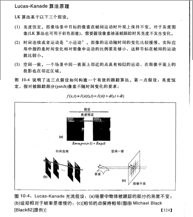
1.首先是假设条件：

（1）亮度恒定，就是同一点随着时间的变化，其亮度不会发生改变。这是基本光流法的假定（所有光流法变种都必须满足），用于得到光流法基本方程；

（2）小运动，这个也必须满足，就是时间的变化不会引起位置的剧烈变化，这样灰度才能对位置求偏导（换句话说，小运动情况下我们才能用前后帧之间单位位置变化引起的灰度变化去近似灰度对位置的偏导数），这也是光流法不可或缺的假定；

（3）空间一致，一个场景上邻近的点投影到图像上也是邻近点，且邻近点速度一致。这是Lucas-Kanade光流法特有的假定，因为光流法基本方程约束只有一个，而要求x，y方向的速度，有两个未知变量。我们假定特征点邻域内做相似运动，就可以连立n多个方程求取x，y方向的速度（n为特征点邻域总点数，包括该特征点）。

2.方程求解

多个方程求两个未知变量，又是线性方程，很容易就想到用最小二乘法，事实上opencv也是这么做的。其中，最小误差平方和为最优化指标。

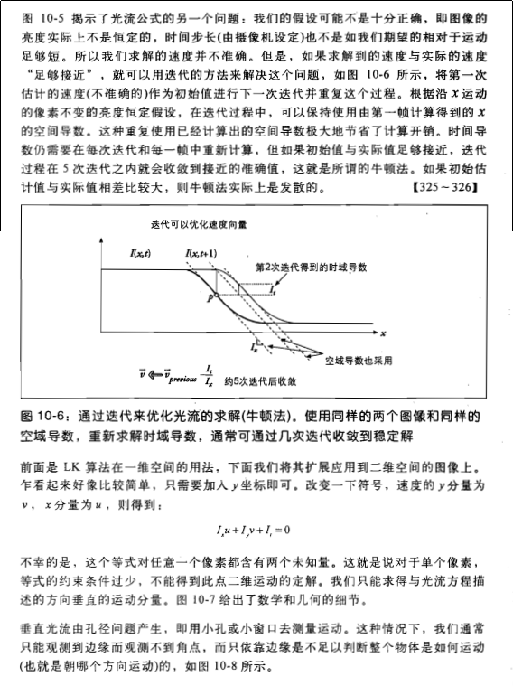
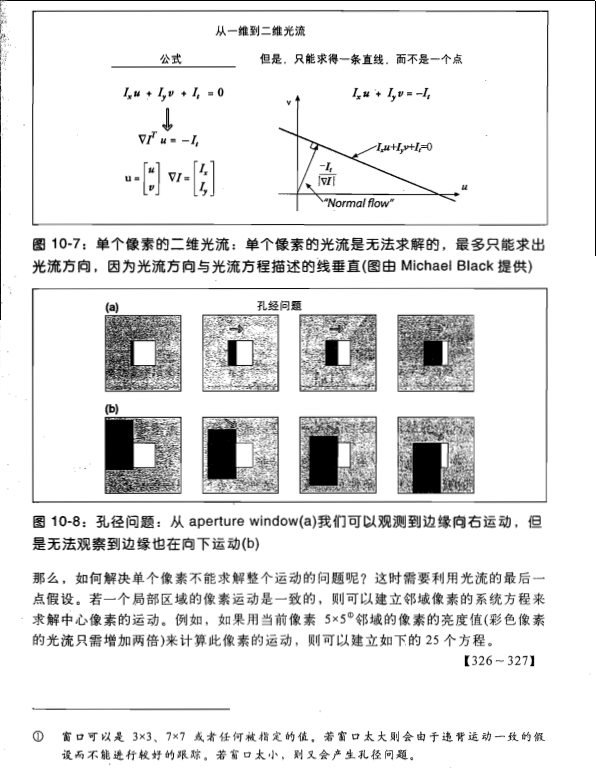
3.好吧，前面说到了小运动这个假定，聪明的你肯定很不爽了，目标速度很快那这货不是二掉了。幸运的是多尺度能解决这个问题。首先，对每一帧建立一个高斯金字塔，最大尺度图片在最顶层，原始图片在底层。然后，从顶层开始估计下一帧所在位置，作为下一层的初始位置，沿着金字塔向下搜索，重复估计动作，直到到达金字塔的底层。聪明的你肯定发现了：这样搜索不仅可以解决大运动目标跟踪，也可以一定程度上解决孔径问题（相同大小的窗口能覆盖大尺度图片上尽量多的角点，而这些角点无法在原始图片上被覆盖）。

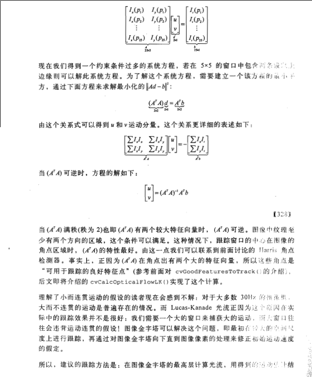
三.opencv中的光流法函数

opencv2.3.1中已经实现了基于光流法的特征点位置估计函数（当前帧位置已知，前后帧灰度已知），介绍如下（摘自opencv2.3.1参考手册）：

calcOpticalFlowPyrLK
Calculates an optical flow for a sparse feature set using the iterative Lucas-Kanade method with pyramids.  

void calcOpticalFlowPyrLK(InputArray prevImg, InputArray nextImg, InputArray prevPts,
InputOutputArray nextPts, OutputArray status, OutputArray err,
Size winSize=Size(15,15), int maxLevel=3, TermCriteria crite-
ria=TermCriteria(TermCriteria::COUNT+TermCriteria::EPS, 30, 0.01),
double derivLambda=0.5, int flags=0 )  

Parameters
prevImg – First 8-bit single-channel or 3-channel input image.
nextImg – Second input image of the same size and the same type as prevImg .
prevPts – Vector of 2D points for which the flow needs to be found. The point coordinates
must be single-precision floating-point numbers.
nextPts – Output vector of 2D points (with single-precision floating-point coordinates)
containing the calculated new positions of input features in the second image. When
OPTFLOW_USE_INITIAL_FLOW flag is passed, the vector must have the same size as in the
input.
status – Output status vector. Each element of the vector is set to 1 if the flow for the
corresponding features has been found. Otherwise, it is set to 0.
err – Output vector that contains the difference between patches around the original and
moved points.
winSize – Size of the search window at each pyramid level.  

maxLevel – 0-based maximal pyramid level number. If set to 0, pyramids are not used
(single level). If set to 1, two levels are used, and so on.
criteria – Parameter specifying the termination criteria of the iterative search algorithm
(after the specified maximum number of iterations criteria.maxCount or when the search
window moves by less than criteria.epsilon .
derivLambda – Not used.  

flags – Operation flags:
– OPTFLOW_USE_INITIAL_FLOW Use initial estimations stored in nextPts . If the
flag is not set, then prevPts is copied to nextPts and is considered as the initial estimate. 

四.用类封装基于光流法的目标跟踪方法

废话少说，附上代码，包括特征点提取，跟踪特征点，标记特征点等。

<span style="font-size:18px;">//帧处理基类
class FrameProcessor{
public:
virtual void process(Mat &input,Mat &ouput)=0;
};  

//特征跟踪类，继承自帧处理基类
class FeatureTracker :  public FrameProcessor{
    Mat gray;  //当前灰度图
    Mat gray_prev;  //之前的灰度图
    vector<Point2f> points[2];//前后两帧的特征点
    vector<Point2f> initial;//初始特征点
    vector<Point2f> features;//检测到的特征
int max_count; //要跟踪特征的最大数目
double qlevel; //特征检测的指标
double minDist;//特征点之间最小容忍距离
    vector<uchar> status; //特征点被成功跟踪的标志
    vector<float> err; //跟踪时的特征点小区域误差和
public:
    FeatureTracker():max_count(500),qlevel(0.01),minDist(10.){}
void process(Mat &frame,Mat &output){
//得到灰度图
        cvtColor (frame,gray,CV_BGR2GRAY);
        frame.copyTo (output);
//特征点太少了，重新检测特征点
if(addNewPoint()){
            detectFeaturePoint ();
//插入检测到的特征点
            points[0].insert (points[0].end (),features.begin (),features.end ());
            initial.insert (initial.end (),features.begin (),features.end ());
        }
//第一帧
if(gray_prev.empty ()){
                gray.copyTo (gray_prev);
        }
//根据前后两帧灰度图估计前一帧特征点在当前帧的位置
//默认窗口是15*15
        calcOpticalFlowPyrLK (
                gray_prev,//前一帧灰度图
                gray,//当前帧灰度图
                points[0],//前一帧特征点位置
                points[1],//当前帧特征点位置
                status,//特征点被成功跟踪的标志
                err);//前一帧特征点点小区域和当前特征点小区域间的差，根据差的大小可删除那些运动变化剧烈的点
int k = 0;
//去除那些未移动的特征点
for(int i=0;i<points[1].size ();i++){
if(acceptTrackedPoint (i)){
                initial[k]=initial[i];
                points[1][k++] = points[1][i];
            }
        }
        points[1].resize (k);
        initial.resize (k);
//标记被跟踪的特征点
        handleTrackedPoint (frame,output);
//为下一帧跟踪初始化特征点集和灰度图像

转载自：http://www.xuebuyuan.com/2023445.html

matlab 参考程序 如下：

%%% Usage: Lucas_Kanade('1.bmp','2.bmp',10)
%%%%%%%%%%%%%%%%%%%%%%%%%%%%%%%%%%%%%%%%%%%%%%%%%%%%%%%%
%%%file1：输入图像1
%%%file2：输入图像2
%%%density：显示密度
function Lucas_Kanade(file1, file2, density)
%%% Read Images %% 读取图像
img1 = im2double (imread (file1));
%%% Take alternating rows and columns %% 按行分成奇偶
[odd1, ~] = split (img1);
img2 = im2double (imread (file2));
[odd2, ~] = split (img2);
%%% Run Lucas Kanade %% 运行光流估计
[Dx, Dy] = Estimate (odd1, odd2);
%%% Plot %% 绘图
figure;
[maxI,maxJ] = size(Dx);
Dx = Dx(1:density:maxI,1:density:maxJ);
Dy = Dy(1:density:maxI,1:density:maxJ);
quiver(1:density:maxJ, (maxI):(-density):1, Dx, -Dy, 1);
axis square;

%%% Run Lucas Kanade on all levels and interpolate %% 光流
function [Dx, Dy] = Estimate (img1, img2)
level = 4;%%%金字塔层数
half_window_size = 2;
% [m, n] = size (img1);
G00 = img1;
G10 = img2;
if (level > 0)%%%从零到level
    G01 = reduce (G00); G11 = reduce (G10);
end
if (level>1)
    G02 = reduce (G01); G12 = reduce (G11);
end
if (level>2)
    G03 = reduce (G02); G13 = reduce (G12);
end
if (level>3)
    G04 = reduce (G03); G14 = reduce (G13);
end
l = level;

for i = level: -1 :0,
    if (l == level)
        switch (l)
        case 4, Dx = zeros (size (G04)); Dy = zeros (size (G04));
        case 3, Dx = zeros (size (G03)); Dy = zeros (size (G03));
        case 2, Dx = zeros (size (G02)); Dy = zeros (size (G02));
        case 1, Dx = zeros (size (G01)); Dy = zeros (size (G01));
        case 0, Dx = zeros (size (G00)); Dy = zeros (size (G00));
        end
    else
        Dx = expand (Dx);
        Dy = expand (Dy);
        Dx = Dx .* 2;
        Dy = Dy .* 2;
    end
    switch (l)
    case 4,
        W = warp (G04, Dx, Dy);
        [Vx, Vy] = EstimateMotion (W, G14, half_window_size);
    case 3,
        W = warp (G03, Dx, Dy);
        [Vx, Vy] = EstimateMotion (W, G13, half_window_size);
    case 2,
        W = warp (G02, Dx, Dy);
        [Vx, Vy] = EstimateMotion (W, G12, half_window_size);
    case 1,
        W = warp (G01, Dx, Dy);
        [Vx, Vy] = EstimateMotion (W, G11, half_window_size);
    case 0,
        W = warp (G00, Dx, Dy);
        [Vx, Vy] = EstimateMotion (W, G10, half_window_size);
    end
    [m, n] = size (W);
    Dx(1:m, 1:n) = Dx(1:m,1:n) + Vx; Dy(1:m, 1:n) = Dy(1:m, 1:n) + Vy;
    smooth (Dx);
    smooth (Dy);
    l = l - 1;
end

%%% Lucas Kanade on the image sequence at pyramid step %%
function [Vx, Vy] = EstimateMotion (W, G1, half_window_size)
[m, n] = size (W);
Vx = zeros (size (W)); Vy = zeros (size (W));
N = zeros (2*half_window_size+1, 5);
for i = 1:m,
    l = 0;
    for j = 1-half_window_size:1+half_window_size,
        l = l + 1;
        N (l,:) = getSlice (W, G1, i, j, half_window_size);
    end
    replace = 1;
    for j = 1:n,
        t = sum (N);
        [v, d] = eig ([t(1) t(2);t(2) t(3)]);
        namda1 = d(1,1); namda2 = d(2,2);
        if (namda1 > namda2)
            tmp = namda1; namda1 = namda2; namda2 = tmp;
            tmp1 = v (:,1); v(:,1) = v(:,2); v(:,2) = tmp1;
        end
        if (namda2 < 0.001)
            Vx (i, j) = 0; Vy (i, j) = 0;
        elseif (namda2 > 100 * namda1)
            n2 = v(1,2) * t(4) + v(2,2) * t(5);
            Vx (i,j) = n2 * v(1,2) / namda2;
            Vy (i,j) = n2 * v(2,2) / namda2;
        else
            n1 = v(1,1) * t(4) + v(2,1) * t(5);
            n2 = v(1,2) * t(4) + v(2,2) * t(5);
            Vx (i,j) = n1 * v(1,1) / namda1 + n2 * v(1,2) / namda2;
            Vy (i,j) = n1 * v(2,1) / namda1 + n2 * v(2,2) / namda2;
        end
        N (replace, :) = getSlice (W, G1, i, j+half_window_size+1, half_window_size);
        replace = replace + 1;
        if (replace == 2 * half_window_size + 2)
            replace = 1;
        end
    end
end

%%% The Reduce Function for pyramid %%金字塔压缩
function result = reduce (ori)
[m,n] = size (ori);
mid = zeros (m, n);
%%%行列值的一半
m1 = round (m/2);
n1 = round (n/2);
%%%输出即为输入图像的1/4
result = zeros (m1, n1);
%%%滤波
%%%0.05  0.25  0.40  0.25  0.05
w = generateFilter (0.4);
for j = 1 : m,
   tmp = conv([ori(j,n-1:n) ori(j,1:n) ori(j,1:2)], w);
   mid(j,1:n1) = tmp(5:2:n+4);
end
for i=1:n1,
   tmp = conv([mid(m-1:m,i); mid(1:m,i); mid(1:2,i)]', w);
   result(1:m1,i) = tmp(5:2:m+4)';
end

%%% The Expansion Function for pyramid %%金字塔扩展
function result = expand (ori)
[m,n] = size (ori);
mid = zeros (m, n);
%%%行列值的两倍
m1 = m * 2;
n1 = n * 2;
%%%输出即为输入图像的4倍
result = zeros (m1, n1);
%%%滤波
%%%0.05  0.25  0.40  0.25  0.05
w = generateFilter (0.4);
for j=1:m,
   t = zeros (1, n1);
   t(1:2:n1-1) = ori (j,1:n);
   tmp = conv ([ori(j,n) 0 t ori(j,1) 0], w);
   mid(j,1:n1) = 2 .* tmp (5:n1+4);
end
for i=1:n1,
   t = zeros (1, m1);
   t(1:2:m1-1) = mid (1:m,i)';
   tmp = conv([mid(m,i) 0 t mid(1,i) 0], w);
   result(1:m1,i) = 2 .* tmp (5:m1+4)';
end

function filter = generateFilter (alpha)%%%滤波系数
filter = [0.25-alpha/2, 0.25, alpha, 0.25, 0.25-alpha/2];

function [N] = getSlice (W, G1, i, j, half_window_size)
N = zeros (1, 5);
[m, n] = size (W);
for y = -half_window_size:half_window_size,
    Y1 = y +i;
    if (Y1 < 1)
        Y1 = Y1 + m;
    elseif (Y1 > m)
        Y1 = Y1 - m;
    end
    X1 = j;
    if (X1 < 1)
        X1 = X1 + n;
    elseif (X1 > n)
        X1 = X1 - n;
    end
    DeriX = Derivative (G1, X1, Y1, 'x'); %%%计算x、y方向梯度
    DeriY = Derivative (G1, X1, Y1, 'y');
    N = N + [ DeriX * DeriX, ...
        DeriX * DeriY, ...
        DeriY * DeriY, ...
        DeriX * (G1 (Y1, X1) - W (Y1, X1)), ...
        DeriY * (G1 (Y1, X1) - W (Y1, X1))];
end

function result = smooth (img)
result = expand (reduce (img));%%%太碉

function [odd, even] = split (img)
[m, ~] = size (img);%%%按行分成奇偶
odd = img (1:2:m, :);
even = img (2:2:m, :);

%%% Interpolation %% 插值
function result = warp (img, Dx, Dy)
[m, n] = size (img);
[x,y] = meshgrid (1:n, 1:m);
x = x + Dx (1:m, 1:n);
y = y + Dy (1:m,1:n);
for i=1:m,
    for j=1:n,
        if x(i,j)>n
            x(i,j) = n;
        end
        if x(i,j)<1
            x(i,j) = 1;
        end
        if y(i,j)>m
            y(i,j) = m;
        end
        if y(i,j)<1
            y(i,j) = 1;
        end
    end
end
result = interp2 (img, x, y, 'linear');%%%二维数据内插值

%%% Calculates the Fx Fy %% 计算x、y方向梯度
function result = Derivative (img, x, y, direction)
[m, n] = size (img);
switch (direction)
case 'x',
    if (x == 1)
        result = img (y, x+1) - img (y, x);
    elseif (x == n)
        result = img (y, x) - img (y, x-1);
    else
        result = 0.5 * (img (y, x+1) - img (y, x-1));
    end
case 'y',
    if (y == 1)
        result = img (y+1, x) - img (y, x);
    elseif (y == m)
        result = img (y, x) - img (y-1, x);
    else
        result = 0.5 * (img (y+1, x) - img (y-1, x));
    end
end