[C5/C6] 机器学习诊断和系统设计(Machine learning Diagnostic and System Desig

机器学习诊断（Machine learning diagnostic）

Diagnostic : A test that you can run to gain insight what is / isn't working with a learning algorithm, and gain guidance as to how best to improve its performance. Diagnostics can take time to implement, but doing so can be a very good use of your time.

划分数据集（Train / Cross Validation / Test）

一个算法在训练集上拟合的好，但泛化能力未必好。所以可改进一下，将原有训练集重新划分（如果训练集非随机分布，先随机打散，之后再划分，可防止样本数据倾斜）为三个部分（Train Set / Cross Validation Set / Test Set），让算法在相对独立的数据集上 训练 / 交叉验证（泛化）/ 测试：

Training set: 60%
Cross validation set: 20%
Test set: 20%

用误差评估假设（Evaluating a Hypothesis with error）

线性回归 和 逻辑回归 的 cost function 可用来配合求解假设的最优参数 $\Theta$，还可用来评估假设，此时称 J 为误差（error）。

回顾 线性回归 和 逻辑回归 的 cost function：

$J(\theta)=\frac{1}{2m} \Bigg[ \sum\limits_{i=1}^m \Big( h_\theta(x^{(i)}) - y^{(i)} \Big)^2 + \lambda \sum\limits_{j=1}^n \theta_j^2 \Bigg]$

$J(\theta)=-\frac{1}{m} \sum\limits_{i=1}^m \Bigg[ y^{(i)} \cdot log \bigg(h_\theta(x^{(i)}) \bigg) + (1-y^{(i)}) \cdot log \bigg(1-h_\theta(x^{(i)}) \bigg) \Bigg] + \frac{\lambda}{2m} \sum\limits_{j=1}^n \theta_j^2$

对于分类问题（e.g. 逻辑回归），除了使用 J （标准的）来表示误差之外，还可以使用误分率（Misclassification Error）来表示，如下：

$\begin{cases} err(h_{\Theta}(x),y) = \begin{cases} 1 \quad & \text{if } h_\Theta(x) \geq 0.5 \text{ and } y=0 \text{ or } h_\Theta(x) < 0.5 \text{ and } y = 1 \\ 0 \quad & otherwise \end{cases} \\ \\ Error=\frac{1}{m} \sum\limits_{i=1}^{m}err(h_\Theta(x^{(i)}),y^{(i)}) \end{cases}$

三个数据集和误差结合使用

将误差对应到不同的数据集，可对应得到三个误差：

训练误差 ：$Error_{train} = J_{train}$
- 计算方法：使用训练集训练样本，得到 $\Theta$，$\lambda$， 训练误差
交叉验证误差（泛化误差）：$Error_{cv} = J_{cv}$
- 计算方法：使用上面的 $\Theta$，$\lambda$ 在交叉验证集上计算 交叉验证误差
测试误差：$Error_{test} = J_{test}$
- 计算方法：使用上面的 $\Theta$，$\lambda$ 在测试集上计算 测试误差

应用：在不同角度下，观察多种场景对应的 Errors 的变化情况，可监测算法的性能。

举例说明：

从样本的角度来看，我们观察样本数量从1增加到m时，对应的训练误差和交叉验证误差的变化情况，可画出 学习曲线，它可以判断算法是否处于 高偏差 或 高方差 或是 Just Right
从多项式次幂数的角度来看，我们观察不同多项式次幂数时，对应的训练误差和交叉验证误差的变化情况，可画出一个曲线图辅助我们选择最优的多项式次幂数。
从正则化参数 $\lambda$ 的角度来看，我们观察选择不同 $\lambda$ 时，对应的训练误差和交叉验证误差的变化情况，可画出一个曲线图辅助我们选择最优的 $\lambda$。
其他角度同训练误差和交叉验证误差相结合 ... etc.

实际的例子

Suppose your learning algorithm is performing less well than you were hoping.
训练误差很低，但是泛化误差很高，所以你需要优化算法。
对于大多数机器学习需要解决的是以下 两个问题 :

1. 欠拟合（Underfitting），即 高偏差（High Bias）
2. 过拟合（Overfitting），即 高方差（High Variance）

而针对 欠拟合 或 过拟合，有以下 6 种方法 可以用来优化算法和解决对应的问题：

1. Get more training examples -> fixes high variance
2. Try smaller sets of features -> fixes high variance
3. Try getting additional features -> fixes high bias
4. Try adding polynomial features ($x_1^2,x_2^2,x_1x_2,etc.$) -> fixes high bias
5. Try decreasing lambda -> fixes high bias
6. Try increasing lambda -> fixes high variance

学习曲线(Learning curves) 诊断欠拟合 / 过拟合 / 均衡状态

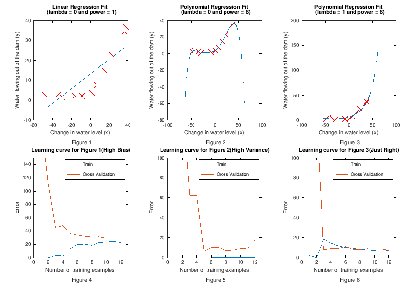
高偏差（Figure 1 和 Figure 4）
Figure 1 为用线性回归拟合数据，Figure 4 为它对应的学习曲线。这是一个高偏差的例子，可以看到：

训练集很少时，训练误差很低，交叉验证（泛化）误差很高
训练集增多时，训练误差和泛化误差近似，但是都居高不下
此时，对于高偏差问题，即使增加再多的训练样本也于事无补

高方差（Figure 2 和 Figure 5）
通过上面的学习曲线，发现算法存在高偏差问题，假定我们决定使用引言中所示的 6种方法 中的第4种（即添加多项式特征）来改善高偏差的情况，假定我们已经选择了 8 次多项式。如下：
Figure 2 为用多项式回归拟合数据，Figure 5 为它对应的学习曲线。这又变成了一个高方差的例子，可以看到：

训练集很少时，训练误差很低，交叉验证（泛化）误差很高
随着训练集增加训练误差升高，泛化误差持续降低但并未持平，且仍和训练误差有很大距离
此时，增加训练样本数量对解决高方差问题非常有帮助，当样本数量到达一定程度，两条线会靠近并持平，且维持在低位。

比较均衡的情况（Figure 3 和 Figure 6）
通过上面的学习曲线，发现算法存在高方差问题，假定我们决定使用引言中所示的 6种方法 中的第6种（即增加正则化参数 $\lambda$）来改善高方差的情况，假定我们已经选择了 $\lambda$ = 1。如下：
Figure 3 为用多项式回归拟合数据，Figure 6 为它对应的学习曲线。这次是一个比较均衡（Just Right）的例子，可以看到：随着训练样本增加，训练误差和泛化误差非常接近，并且处于很低的位置。

以下为三个学习曲线的绘图数据，可供参考：

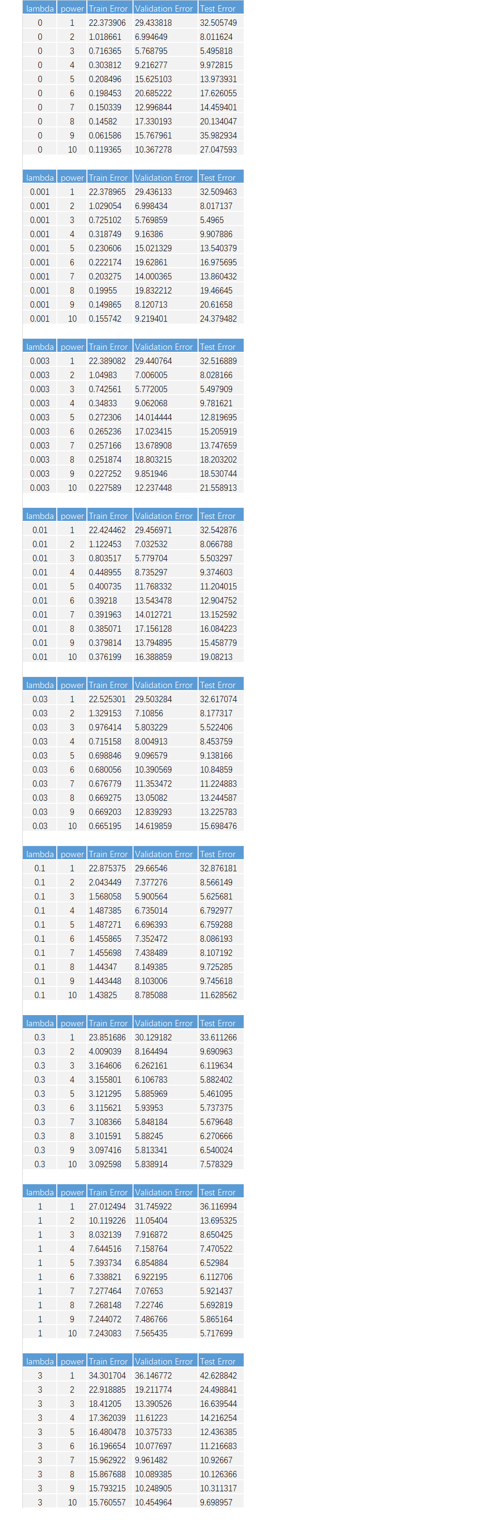
模型选择曲线（Model Selection curves）

这里展开说明一下，上面例子中多项式次幂数 = 8 和 $\lambda$ = 1 的由来。

上面 9 张图对应 9 个 $\lambda$ 的值，其中每张图中，x轴为多项式次数从1 ~ 10，y轴为 Error，两条线分别为训练误差和交叉验证（泛化）误差。

可以看到

9 张图中，只有当 $\lambda$ = 1 时，训练误差和泛化误差最为接近，且维持在一个低位。
当 $\lambda$ = 1 时，只有多项式次数为 8 的时候，训练误差和泛化误差最为接近（有个交叉），且维持在一个低位，同时测试误差也非常低。此处结合画图所用的数据来观察更为直观一些，下面会给出具体的用来绘制 9 张图的数据信息。

Diagnosing Neural Networks

A neural network with fewer parameters is prone to underfitting.
It is also computationally cheaper.

A large neural network with more parameters is prone to overfitting.
It is also computationally expensive.
In this case you can use regularization (increase λ) to address the overfitting.

Using a single hidden layer is a good starting default.
You can train your neural network on a number of hidden layers using your cross validation set.
You can then select the one that performs best.

程序代码

直接查看Machine Learning Diagnostics & Bias-Variance & Learning Curve.ipynb可点击

获取源码以其他文件，可点击右上角 Fork me on GitHub 自行 Clone。

机器学习系统设计（Machine Learning System Design）

To optimize a machine learning algorithm, you’ll need to first understand where the biggest improvements can be made. In this module, we discuss how to understand the performance of a machine learning system with multiple parts, and also how to deal with skewed data.

Build Machine Learning System

The recommended approach to solving machine learning problems is to:

Start with a simple algorithm, implement it quickly, and test it early on your cross validation data.
Plot learning curves to decide if more data, more features, etc. are likely to help.
Manually examine the errors on examples in the cross validation set and try to spot a trend where most of the errors were made.

For example, assume that we have 500 emails and our algorithm misclassifies a 100 of them. We could manually analyze the 100 emails and categorize them based on what type of emails they are. We could then try to come up with new cues and features that would help us classify these 100 emails correctly. Hence, if most of our misclassified emails are those which try to steal passwords, then we could find some features that are particular to those emails and add them to our model. We could also see how classifying each word according to its root changes our error rate.

It is very important to get error results as a single, numerical value. Otherwise it is difficult to assess your algorithm's performance. For example if we use stemming, which is the process of treating the same word with different forms (fail/failing/failed) as one word (fail), and get a 3% error rate instead of 5%, then we should definitely add it to our model. However, if we try to distinguish between upper case and lower case letters and end up getting a 3.2% error rate instead of 3%, then we should avoid using this new feature. Hence, we should try new things, get a numerical value for our error rate, and based on our result decide whether we want to keep the new feature or not.

To deal with skewed classes data

在训练机器学习算法时，可能会遇到倾斜类的训练数据，比如，在癌症诊断时，医学上来说可能只有 0.5% 的样本是患有癌症的。假如此时算法误差为 1%，如果预测所有样本为非患有癌症，那么误差反而提高到 0.5%，但这么做显然是不可取的。

查准率和查全率

引入两个比率来度量上面提到的情况，查准率（精确度 / Precision ）和 查全率（召回率 / Recall）

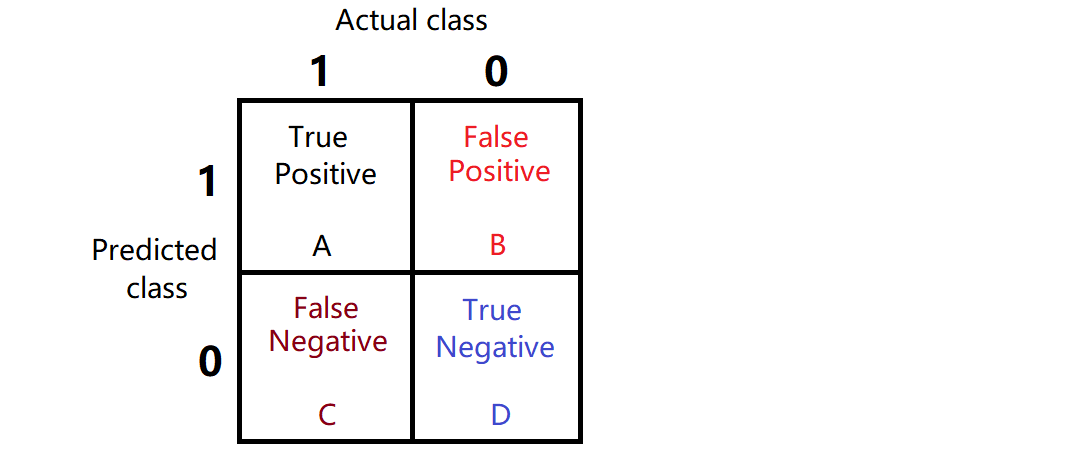
查准率（P） = $\frac{A}{A+B}$，Intuition：所有算法预测为 1 的样本中，正确的比率
查全率（R） = $\frac{A}{A+C}$，Intuition：所有为 1 的样本中，算法预测正确的比率

以上面判断癌症的样本为例，假定有 100 个样本，其中 5 个 1 样本，95 个 0 样本：

绝对理想状态，A = 5, B = C = 0, D = 95。 P = R = 100%
准确率 100%, 召回率 100%，说明预测绝对的准确，一个错判都没有。而且样本中所有为 1 的样本都被成功预测出来(召回)了
全部预测为 0，那么 P = R = 0
虽然误差只有 0.5%，但是从 P 和 R 的度量角度（同等于0），可以暴露出算法问题。
全部预测为 1，那么 P = 0.5%， R = 100%
召回率 100%，说明所有为 1 的样本都被算法预测出来了，但是因为恒预测 1，C 和 D肯定都是 0，而 A = 5，B = 95，这样查准率为 0.5%， P 和 R 差距太大，同样暴露算法问题。
如果改变预测为 1 的阈(yù)值 50% → 70%, then B↘ and C↗，so P↗ and R↘
如果改变预测为 1 的阈(yù)值 50% → 30%, then B↗ and C↘，so P↘ and R↗
4 和 5，为人为调节查准率和查全率比重的情况。例如在商品推荐系统中，为了尽可能少打扰用户，更希望推荐内容确实是用户感兴趣的，此时会酌情提高查准率；而在逃犯信息检索系统中，更希望尽可能少漏掉逃犯，此时会刻意提高查全率。

P 与 R 是互斥的，一个升高另一个就会跟着降低。可以根据实际需求人为设置阈值，但更一般情况下，还是希望 P 和 R 可以均衡一些。对于非人为不均衡的情况，需要警惕算法是否存在问题（e.g. 设置恒预测 0 时）。

可以使用 P-R曲线来直观的展示 P 和 R 的联动变化情况。

P-R曲线

设置三个不同的阈值，计算出查准率和查全率，可绘制出以下 P-R图 :

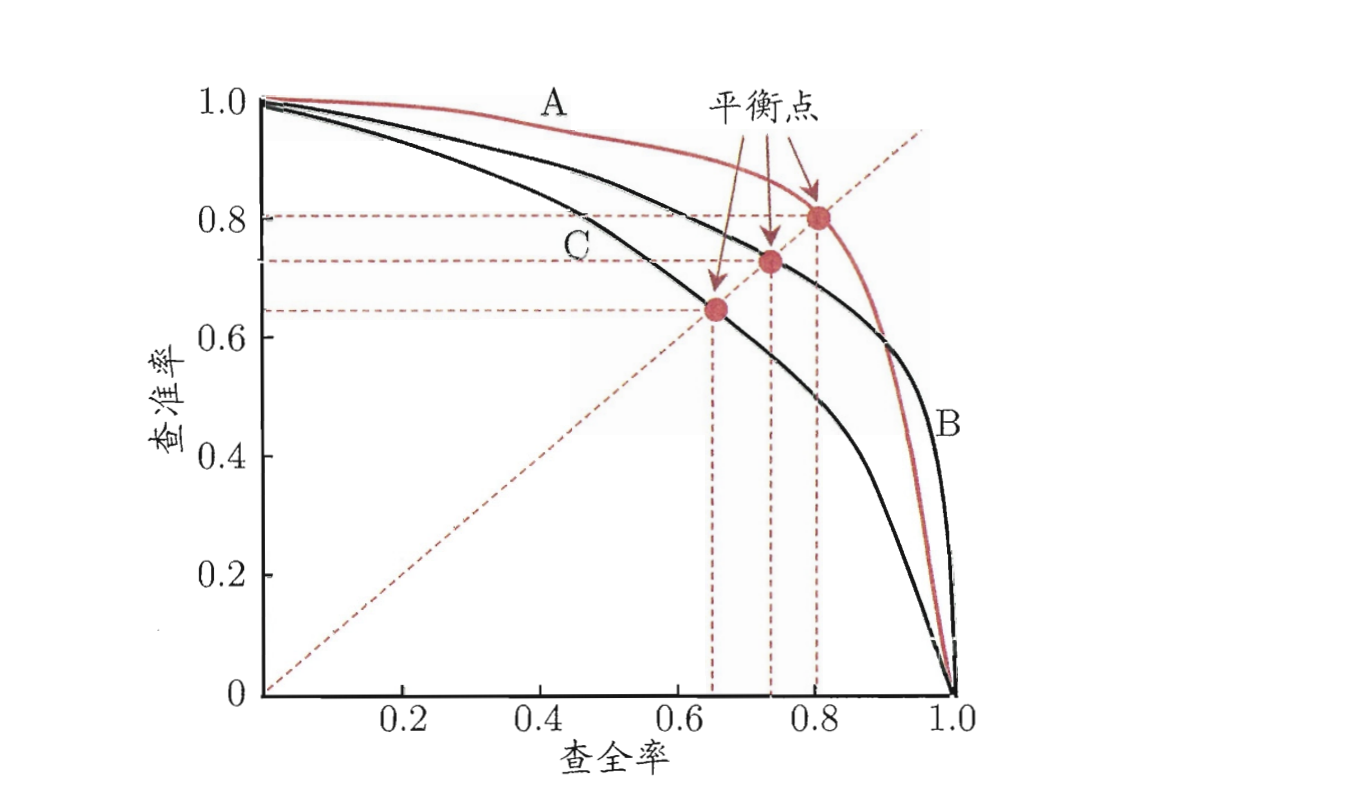
查准率和查全率的最大边界值都为 1 ，即 100%。
图中曲线 B 完全包裹注 C，所以性能 B 大于 C。
图中曲线 A 和 B 有交叉点，可比较曲线下方面积大小，面积大性能好。缺点为不容易计算。

因此，需要引入新的度量来判断曲线性能，比如 BEP 和 F1

平衡点(BEP)

平衡点（Break-Even-Point） = 当 "查准率=查全率" 时的取值

根据BEP可判断上图中曲线性能： A > B > C

F1度量

相比过于简单的 BEP 度量，更为通用的是 $F_1$ 度量。

$\frac{1}{F_\beta} = \frac{1}{1 + \beta^2}\big( \frac{1}{P} + \frac{\beta^2}{R} \big)$

加权调和平均比算术平均 $\frac{P+R}{2}$ 和几何平均 $(\sqrt{P+R})$ 更加重视较小值。

当 $\beta$ = 1 时，此时它的定义是基于查准率与查全率的调和平均，公式如下：

$\frac{1}{F_1} = \frac{1}{2}\big( \frac{1}{P} + \frac{1}{R} \big)$

对上面公式取倒数，即得 $F_1$ 度量公式，如下：

$F_1 = 2\frac{PR}{P + R} = \frac{2 \times TP}{m + TP - TN}$

在一些应用中，对查准率和查全率的重视程度有所不同。例如：

在商品推荐系统中，为了尽可能少打扰用户，更希望推荐内容确实是用户感兴趣的，此时查准率更重要；
而在逃犯信息检索系统中，更希望尽可能少漏掉逃犯，此时查全率更重要。

F 度量的一般形式可表达出对查准率 / 查全率的不同偏好，公式如下：

$F_\beta = \frac{(1 + \beta^2) \times{} P \times{} R}{\beta^2 \times{} P + R}$

不同的 $\beta$ 取值，可表达出 查全率 vs. 查准率 不同的相对重要性：

当 $\beta$ = 1时，退化为标准的 $F_1$
当 $\beta$ > 1时，对查全率有更大影响
当 0 < $\beta$ < 1时，对查准率有更大影响

Data For Machine Learning

某些情况下，如果训练样本充足，"劣等算法" 可优于具有较少训练样本的高级算法。
假定有一个低偏差的算法，它是一个有很多特征量或隐藏单元的复杂函数，使用大训练集，将减少过拟合的可能性。

In order to have a high performance learning algorithm we want it not to have high bias and not to have high variance. So the bias problem we're going to address by making sure we have a learning algorithm with many parameters and so that gives us a low bias algorithm and by using a very large training set, this ensures that we don't have a variance problem here. So is by pulling these two together, that we end up with a low bias and a low variance learning algorithm and this allows us to do well on the test set.

And fundamentally it's a key ingredients of assuming that the features have enough information and we have a rich class of functions that's why it guarantees low bias, and then it having a massive training set what guarantees more variance.

So this gives us a set of conditions rather hopefully some understanding of what's the sort of problem where if you have a lot of data and you train a learning algorithm with lot of parameters, that might be a good way to give a high performance learning algorithm.

I think the key point that I often ask myself are

first, can a human experts look at the features x and confidently predict the value of y.
Because that's sort of a certification that y can be predicted accurately from the features x.

second, can we actually get a large training set, and train the learning algorithm with a lot of parameters in the training set.

If you can do both then that's more often give you a very kind performance learning algorithm.