Python Machine Learning-Chapter4
Chapter4 Building Good Training Sets – Data Preprocessing
4.1 Dealing with missing data
如何判断数据框内的数据是否有空值呢?
import pandas as pd

from io import StringIO

csv_data = '''A, B, C, D

1.0,2.0,3.0,4.0

5.0,6.0,,8.0

10.0,11.0,12.0,'''

df = pd.read_csv(StringIO(csv_data))

df.isnull()

'''

 A      B      C      D

0  False  False  False  False

1  False  False   True  False

2  False  False  False   True

'''

df.isnull().sum()

'''

A    0

B    0

C    1

D    1

dtype: int64
4.2 Eliminating samples or features with missing values
既可以去除含NA的行,也可以去除含NA的列
import pandas as pd

from io import StringIO

csv_data = '''A, B, C, D

1.0,2.0,3.0,4.0

5.0,6.0,,8.0

10.0,11.0,12.0,'''

df = pd.read_csv(StringIO(csv_data), names=['A', 'B', 'C', 'D'], header=0)

df

'''

        A     B     C    D

0   1.0   2.0   3.0  4.0

1   5.0   6.0   NaN  8.0

2  10.0  11.0  12.0  NaN

'''

df.dropna()#去除含NaN的行

'''

     A    B    C    D

0  1.0  2.0  3.0  4.0

'''

df.dropna(axis=1)#axis参数设置去除NA列

'''

      A     B

0   1.0   2.0

1   5.0   6.0

2  10.0  11.0

'''

# only drop rows where all columns are NaN

df.dropna(how='all')

# drop rows that have not at least 4 non-NaN values至少thresh个非NA的行才被保留

df.dropna(thresh=4)

'''

     A    B    C    D

0  1.0  2.0  3.0  4.0

'''

# only drop rows where NaN appear in specific columns (here: 'C')

df.dropna(subset=['C'])

'''

      A     B     C    D

0   1.0   2.0   3.0  4.0

2  10.0  11.0  12.0  NaN

'''
4.3 Imputing missing values
可以对NaN进行填充,用平均值或者出现次数最多的数据进行填充
import pandas as pd

from io import StringIO

csv_data = '''A,B,C,D

1.0,2.0,3.0,4.0

5.0,6.0,,8.0

10.0,11.0,12.0,'''

df = pd.read_csv(StringIO(csv_data), names=['A','B', 'C', 'D'], header=0)

from sklearn.preprocessing import Imputer

imr = Imputer(missing_values='NaN', strategy='mean', axis=0)

#strategy = 'most_frequent'用出现次数最多的数据填充NaN

#axis = 1 行的平均值填充NaN

imr = imr.fit(df)

df.values

'''

array([[ 1.,  2.,  3.,  4.],

       [ 5.,  6., nan,  8.],

       [10., 11., 12., nan]])

'''

imputed_data = imr.transform(df.values)

imputed_data

'''

array([[ 1. ,  2. ,  3. ,  4. ],

       [ 5. ,  6. ,  7.5,  8. ],

       [10. , 11. , 12. ,  6. ]])

'''
4.4 Handling categorical data and Mapping ordinal features
有的特征虽然不是数值型的,但是也有大小之分,比如T-shirt,XL > L > M,这样的特征称为Ordinal features,而单纯的字符串型特征称为nominal features,先创建一个新的数据框来说明这个问题:
import pandas as pd

df = pd.DataFrame([

    ['green', 'M', 10.1, 'class1'],

    ['red', 'L', 13.5, 'class2'],

    ['blue', 'XL', 15.3, 'class1'] ])

df

'''

       0   1     2       3

0  green   M  10.1  class1

1    red   L  13.5  class2

2   blue  XL  15.3  class1

'''

df.columns = ['color', 'size', 'price', 'classlabel']

df

'''

   color size  price classlabel

0  green    M   10.1     class1

1    red    L   13.5     class2

2   blue   XL   15.3     class1

'''
其中包含nominal feature (color), an ordinal feature (size) and a numerical feature (price),虽然ordinal feature不是数值型,但是也有大小之分,所以需要转换成数值型的特征,现在没有现成的方法完成转换,需要我们自己进行Mapping:
import pandas as pd

df = pd.DataFrame([

    ['green', 'M', 10.1, 'class1'],

    ['red', 'L', 13.5, 'class2'],

    ['blue', 'XL', 15.3, 'class1'] ])

df

'''

       0   1     2       3

0  green   M  10.1  class1

1    red   L  13.5  class2

2   blue  XL  15.3  class1

'''

df.columns = ['color', 'size', 'price', 'classlabel']

df

'''

       0   1     2       3

0  green   M  10.1  class1

1    red   L  13.5  class2

2   blue  XL  15.3  class1

'''

size_mapping = {'XL' :3, 'L':2, 'M':1}#XL = L +1 = M + 2

df['size'] = df['size'].map(size_mapping)

df

'''

   color  size  price classlabel

0  green     1   10.1     class1

1    red     2   13.5     class2

2   blue     3   15.3     class1

'''

#也可以转回去,把数字型转换为字符型

str_mapping = {v:k for k,v in size_mapping.items()}

df['size'] = df['size'].map(str_mapping)

df

'''

   color size  price classlabel

0  green    M   10.1     class1

1    red    L   13.5     class2

2   blue   XL   15.3     class1

'''
许多机器学习算法库要求class label是数值型的,参考上面的mapping方法对class label进行数值转换
import pandas as pd

df = pd.DataFrame([

    ['green', 'M', 10.1, 'class1'],

    ['red', 'L', 13.5, 'class2'],

    ['blue', 'XL', 15.3, 'class1'] ])

df

'''

       0   1     2       3

0  green   M  10.1  class1

1    red   L  13.5  class2

2   blue  XL  15.3  class1

'''

df.columns = ['color', 'size', 'price', 'classlabel']

df

'''

       0   1     2       3

0  green   M  10.1  class1

1    red   L  13.5  class2

2   blue  XL  15.3  class1

'''

size_mapping = {'XL' :3, 'L':2, 'M':1}#XL = L +1 = M + 2

df['size'] = df['size'].map(size_mapping)

df

'''

   color  size  price classlabel

0  green     1   10.1     class1

1    red     2   13.5     class2

2   blue     3   15.3     class1

'''

#也可以转回去,把数字型转换为字符型

str_mapping = {v:k for k,v in size_mapping.items()}

df['size'] = df['size'].map(str_mapping)

df

'''

   color size  price classlabel

0  green    M   10.1     class1

1    red    L   13.5     class2

2   blue   XL   15.3     class1

'''

import numpy as np

class_mapping = {label:idx for idx, label in enumerate(np.unique(df['classlabel']))}

class_mapping

'''

{'class1': 0, 'class2': 1}

'''

df['classlabel'] = df['classlabel'].map(class_mapping)

df

'''

   color size  price  classlabel

0  green    M   10.1         0

1    red    L   13.5         1

2   blue    XL  15.3         0

'''

#也可以转回去,将数字型label转换为字符型

inv_class_mapping = {v: k for k, v in class_mapping.items()}

df['classlabel'] = df['classlabel'].map(inv_class_mapping)

df

'''

   color size  price classlabel

0  green    M   10.1     class1

1    red      L   13.5     class2

2   blue     XL  15.3     class1

'''
当然sklearn有内置的方法(LabelEncoder class)进行label数字型和字符型互相转换:
import pandas as pd

df = pd.DataFrame([

    ['green', 'M', 10.1, 'class1'],

    ['red', 'L', 13.5, 'class2'],

    ['blue', 'XL', 15.3, 'class1'] ])

df

'''

       0   1     2       3

0  green   M  10.1  class1

1    red   L  13.5  class2

2   blue  XL  15.3  class1

'''

df.columns = ['color', 'size', 'price', 'classlabel']

df

'''

       0   1     2       3

0  green   M  10.1  class1

1    red   L  13.5  class2

2   blue  XL  15.3  class1

'''

size_mapping = {'XL' :3, 'L':2, 'M':1}#XL = L +1 = M + 2

df['size'] = df['size'].map(size_mapping)

df

'''

   color  size  price classlabel

0  green     1   10.1     class1

1    red     2   13.5     class2

2   blue     3   15.3     class1

'''

#也可以转回去,把数字型转换为字符型

str_mapping = {v:k for k,v in size_mapping.items()}

df['size'] = df['size'].map(str_mapping)

df

'''

   color size  price classlabel

0  green    M   10.1     class1

1    red    L   13.5     class2

2   blue   XL   15.3     class1

'''

from sklearn.preprocessing import LabelEncoder

class_le = LabelEncoder()

y = class_le.fit_transform(df['classlabel'].values)

y

'''

array([0, 1, 0], dtype=int64)

'''

class_le.inverse_transform(y)

'''

array(['class1', 'class2', 'class1'], dtype=object)

'''
4.5 Performing one-hot encoding on nominal features
nominal feature同样需要进行encode转换成数值,但是如果采用和ordinal feature同样的处理方式:
#coding=utf-8

import pandas as pd

df = pd.DataFrame([

    ['green', 'M', 10.1, 'class1'],

    ['red', 'L', 13.5, 'class2'],

    ['blue', 'XL', 15.3, 'class1'] ])

df.columns = ['color', 'size', 'price', 'classlabel']

size_mapping = {'XL' :3, 'L':2, 'M':1}#XL = L +1 = M + 2

df['size'] = df['size'].map(size_mapping)

df

'''

   color  size  price classlabel

0  green     1   10.1     class1

1    red     2   13.5     class2

2   blue     3   15.3     class1

'''

from sklearn.preprocessing import LabelEncoder

class_le = LabelEncoder()

y = class_le.fit_transform(df['classlabel'].values)

y#array([0, 1, 0], dtype=int64)

'''

#也可以转回去

class_le.inverse_transform(y)

array(['class1', 'class2', 'class1'], dtype=object)

'''

X = df[['color', 'size', 'price']].values

color_le = LabelEncoder()

X[:, 0]  = color_le.fit_transform(X[:, 0])

X

'''

array([[1, 1, 10.1],

       [2, 2, 13.5],

       [0, 3, 15.3]], dtype=object)

blue -> 0

green -> 1

red -> 2

'''
如果把这样的数据给模型训练,模型会认为green特征大于blue,red特征大于green特征,这明显是错误的,所以nominal特征不能采用和ordinal特征一样的处理方式。处理nominal features常用的方法是one-hot encoding,如将color特征变成多维特征,如a blue sample can be encoded as blue=1, green=0, red=0:OneHot Encoder 内置于sklearn.preprocessing中:
#coding=utf-8

import pandas as pd

df = pd.DataFrame([

    ['green', 'M', 10.1, 'class1'],

    ['red', 'L', 13.5, 'class2'],

    ['blue', 'XL', 15.3, 'class1'] ])

df.columns = ['color', 'size', 'price', 'classlabel']

size_mapping = {'XL' :3, 'L':2, 'M':1}#XL = L +1 = M + 2

df['size'] = df['size'].map(size_mapping)

df

'''

   color  size  price classlabel

0  green     1   10.1     class1

1    red     2   13.5     class2

2   blue     3   15.3     class1

'''

from sklearn.preprocessing import LabelEncoder

class_le = LabelEncoder()

y = class_le.fit_transform(df['classlabel'].values)

y#array([0, 1, 0], dtype=int64)


'''

#也可以转回去

class_le.inverse_transform(y)

array(['class1', 'class2', 'class1'], dtype=object)

'''

X = df[['color', 'size', 'price']].values

color_le = LabelEncoder()

X[:, 0] = color_le.fit_transform(X[:, 0])

from sklearn.preprocessing import OneHotEncoder

ohe = OneHotEncoder(categorical_features=[0])

print(ohe.fit_transform(X).toarray())

'''

array([[ 0. ,  1. ,  0. ,  1. , 10.1],

       [ 0. ,  0. ,  1. ,  2. , 13.5],

       [ 1. ,  0. ,  0. ,  3. , 15.3]])

'''

#更常用的one-hot encoding方法是利用pandas中的get_dummies方法,get_dummies方法会只对string columns进行ond-hot encoding,而其他columns不会更改

pd.get_dummies(df[['price', 'color', 'size']])

'''

   price  size  color_blue  color_green  color_red

0   10.1     1           0            1          0

1   13.5     2           0            0          1

2   15.3     3           1            0          0

'''
categorical_features参数指定变量的列(想要进行one-hot encoding的特征位置),而transform方法返回一个稀疏矩阵。
4.6 Partitioning a dataset in training and test sets
#coding=utf-8

import pandas as pd

import numpy as np

df_wine = pd.read_csv('https://archive.ics.uci.edu/ml/machine-learning-databases/wine/wine.data', header=None)

df_wine.columns =[

                                                  'Class label', 'Alcohol',

                                                  'Malic acid', 'Ash',

                                                  'Alcalinity of ash', 'Magnesium',

                                                  'Total phenols', 'Flavanoids',

                                                  'Nonflavanoid phenols',

                                                  'Proanthocyanins',

                                                  'Color intensity', 'Hue',

                                                  'OD280/OD315 of diluted wines',

                                                  'Proline'

                                        ]

print("Class labels", np.unique(df_wine['Class label']))

print(df_wine.head())

from sklearn.cross_validation import train_test_split

X, y = df_wine.iloc[:, 1:].values, df_wine.iloc[:, 0].values#通过行号,列号获取数据

X_train, X_test, y_train, y_test = train_test_split(X, y, test_size=0.3, random_state=0)

print(X,y)
4.7 Bringing features onto the same scale
数据标准化:normalization和standardization
normalization:\( x_{norm} = (x-x_{min})/(x_{max}-x_{min}) \),sklearn.preprocessing中的MinMaxScaler方法可以进行normalization
#coding=utf-8

import pandas as pd

import numpy as np

df_wine = pd.read_csv('https://archive.ics.uci.edu/ml/machine-learning-databases/wine/wine.data', header=None)

df_wine.columns =[

                                                  'Class label', 'Alcohol',

                                                  'Malic acid', 'Ash',

                                                  'Alcalinity of ash', 'Magnesium',

                                                  'Total phenols', 'Flavanoids',

                                                  'Nonflavanoid phenols',

                                                  'Proanthocyanins',

                                                  'Color intensity', 'Hue',

                                                  'OD280/OD315 of diluted wines',

                                                  'Proline'

                                        ]

print("Class labels", np.unique(df_wine['Class label']))

print(df_wine.head())

from sklearn.cross_validation import train_test_split

X, y = df_wine.iloc[:, 1:].values, df_wine.iloc[:, 0].values#通过行号,列号获取数据

X_train, X_test, y_train, y_test = train_test_split(X, y, test_size=0.3, random_state=0)

from sklearn.preprocessing import MinMaxScaler

mms = MinMaxScaler()

X_train_norm = mms.fit_transform(X_train)

X_test_norm = mms.transform(X_test)

print(X_train_norm, X_test_norm)
standardization:\( x_{std} = (x - \mu_{x})/\sigma_x \),其中\( \mu_{x}\)是某特征的mean,\( \sigma_x\)是某特征的standard deviation:
#coding=utf-8

import pandas as pd

import numpy as np

df_wine = pd.read_csv('https://archive.ics.uci.edu/ml/machine-learning-databases/wine/wine.data', header=None)

df_wine.columns =[

                                                  'Class label', 'Alcohol',

                                                  'Malic acid', 'Ash',

                                                  'Alcalinity of ash', 'Magnesium',

                                                  'Total phenols', 'Flavanoids',

                                                  'Nonflavanoid phenols',

                                                  'Proanthocyanins',

                                                  'Color intensity', 'Hue',

                                                  'OD280/OD315 of diluted wines',

                                                  'Proline'

                                        ]

print("Class labels", np.unique(df_wine['Class label']))

print(df_wine.head())

from sklearn.cross_validation import train_test_split

X, y = df_wine.iloc[:, 1:].values, df_wine.iloc[:, 0].values#通过行号,列号获取数据

X_train, X_test, y_train, y_test = train_test_split(X, y, test_size=0.3, random_state=0)

print("============MinMaxScaler============")

from sklearn.preprocessing import MinMaxScaler

mms = MinMaxScaler()

X_train_norm = mms.fit_transform(X_train)

X_test_norm = mms.transform(X_test)

print(X_train_norm, X_test_norm)

print("============StandardScaler============")

from sklearn.preprocessing import StandardScaler

stdsc = StandardScaler()

X_train_std = stdsc.fit_transform(X_train)

X_test_std = stdsc.transform(X_test)

print(X_train_std,X_test_std)
norm和std方法的差别如下表(考虑输入是0到5):
4.8 Selecting meaningful features
过拟合的解决方法:
- Collect more training data(不现实,训练数据有限)
- Introduce a penalty for complexity via regularization
- Choose a simpler model with fewer parameters
- Reduce the dimensionality of the data
4.9 Sequential feature selection algorithms(时序特征)
主要有两种维度减少的方法:特征选择和特征提取,下面以特征选择为例
#coding=utf-8
import pandas as pd
import numpy as np from sklearn.base import clone
from itertools import combinations
import numpy as np
from sklearn.cross_validation import train_test_split
from sklearn.metrics import accuracy_score class SBS():
def __init__(self, estimator, k_features, scoring=accuracy_score, test_size=0.25, random_state=1):
self.scoring = scoring
self.estimator = clone(estimator)
self.k_features = k_features
self.test_size = test_size
self.random_state = random_state def fit(self, X, y):
X_train, X_test, y_train, y_test = train_test_split(X, y, test_size=self.test_size, random_state=self.random_state)
dim = X_train.shape[1]
self.indices_ = tuple(range(dim))
self.subsets_ = [self.indices_]
score = self._calc_score(X_train, y_train, X_test, y_test, self.indices_)
self.scores_ = [score] while dim > self.k_features:
scores = []
subsets = [] for p in combinations (self.indices_, r=dim-1):
score = self._calc_score(X_train, y_train, X_test, y_test, p) scores.append(score)
subsets.append(p) best = np.argmax(scores)
self.indices_ = subsets[best]
self.subsets_.append(self.indices_)
dim -= 1 self.scores_.append(scores[best]) self.k_score_ = self.scores_[-1] return self def transform(self, X):
return X[:, self.indices_] def _calc_score(self, X_train, y_train, X_test, y_test, indices):
self.estimator.fit(X_train[:, indices], y_train)
y_pred = self.estimator.predict(X_test[:, indices])
score = self.scoring(y_test, y_pred)
return score df_wine = pd.read_csv('https://archive.ics.uci.edu/ml/machine-learning-databases/wine/wine.data', header=None)
df_wine.columns =[
'Class label', 'Alcohol',
'Malic acid', 'Ash',
'Alcalinity of ash', 'Magnesium',
'Total phenols', 'Flavanoids',
'Nonflavanoid phenols',
'Proanthocyanins',
'Color intensity', 'Hue',
'OD280/OD315 of diluted wines',
'Proline'
] print("Class labels", np.unique(df_wine['Class label']))
print(df_wine.head()) from sklearn.cross_validation import train_test_split
X, y = df_wine.iloc[:, 1:].values, df_wine.iloc[:, 0].values#通过行号,列号获取数据
X_train, X_test, y_train, y_test = train_test_split(X, y, test_size=0.3, random_state=0) print("============MinMaxScaler============")
from sklearn.preprocessing import MinMaxScaler
mms = MinMaxScaler()
X_train_norm = mms.fit_transform(X_train)
X_test_norm = mms.transform(X_test)
print(X_train_norm, X_test_norm) print("============StandardScaler============")
from sklearn.preprocessing import StandardScaler
stdsc = StandardScaler()
X_train_std = stdsc.fit_transform(X_train)
X_test_std = stdsc.transform(X_test)
print(X_train_std,X_test_std) from sklearn.neighbors import KNeighborsClassifier
import matplotlib.pyplot as plt
knn = KNeighborsClassifier(n_neighbors=2)
sbs = SBS(knn, k_features=1)
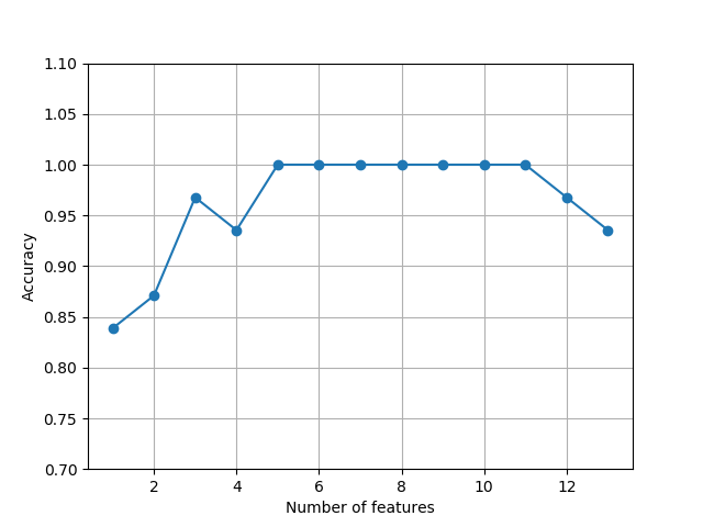
sbs.fit(X_train_std, y_train) #plot the classification accuracy of the KNN classifier that was calculated on the validation dataset.
k_feat = [len(k) for k in sbs.subsets_]
plt.plot(k_feat, sbs.scores_, marker='o')
plt.ylim([0.7, 1.1])
plt.ylabel('Accuracy')
plt.xlabel('Number of features')
plt.grid()
plt.show() #what those five features are that yielded such a good performance on the validation dataset
k5 = list(sbs.subsets_[8])
print(df_wine.columns[1:][k5])#Index(['Alcohol', 'Malic acid', 'Alcalinity of ash', 'Hue', 'Proline'], dtype='object') #let's evaluate the performance of the KNN classifier on the original test set
knn.fit(X_train_std, y_train)
print("Training accuracy:", knn.score(X_train_std, y_train))
#Training accuracy: 0.9838709677419355
print("Test accuracy:", knn.score(X_test_std, y_test))
#Test accuracy: 0.9444444444444444
'''
We used the complete feature set and obtained ~98.4 percent accuracy on the training dataset.
However, the accuracy on the test dataset was slightly lower (~94.4 percent),
which is an indicator of a slight degree of overfitting.
''' #Now let's use the selected 5-feature subset and see how well KNN performs
knn.fit(X_train_std[:, k5], y_train)
print('Training accuracy:', knn.score(X_train_std[:, k5], y_train))
#Training accuracy: 0.9596774193548387
print("Test accuracy:", knn.score(X_test_std[:, k5], y_test))
#Test accuracy: 0.9629629629629629
'''
Using fewer than half of the original features in the Wine dataset, the prediction
accuracy on the test set improved by almost 2 percent. Also, we reduced overfitting,
which we can tell from the small gap between test (~96.3 percent) and training
(~96.0 percent) accuracy.
'''
itertools中的combinations可以帮助我们从一个元组中选择若干个元素,并将其展示出来,如\C_6^2\)
S = ('ABCDEF')

for each in combinations(S, r=2):

    print(each)

#r指定选几个

'''

('A', 'B')

('A', 'C')

('A', 'D')

('A', 'E')

('A', 'F')

('B', 'C')

('B', 'D')

('B', 'E')

('B', 'F')

('C', 'D')

('C', 'E')

('C', 'F')

('D', 'E')

('D', 'F')

('E', 'F')

'''
关于itertools包的使用,可以参考:https://docs.python.org/2/library/itertools.html
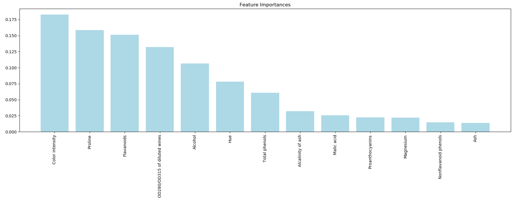
4.10 Assessing feature importance with random forests
Train a forest of 10,000 trees on the Wine dataset and rank the 13 features by their respective importance measures and we don't need to use standardized or normalized tree-based models.
#coding=utf-8

import pandas as pd

import numpy as np

df_wine = pd.read_csv('https://archive.ics.uci.edu/ml/machine-learning-databases/wine/wine.data', header=None)

df_wine.columns =[

                                                  'Class label', 'Alcohol',

                                                  'Malic acid', 'Ash',

                                                  'Alcalinity of ash', 'Magnesium',

                                                  'Total phenols', 'Flavanoids',

                                                  'Nonflavanoid phenols',

                                                  'Proanthocyanins',

                                                  'Color intensity', 'Hue',

                                                  'OD280/OD315 of diluted wines',

                                                  'Proline'

                                        ]

print("Class labels", np.unique(df_wine['Class label']))

print(df_wine.head())

from sklearn.cross_validation import train_test_split

X, y = df_wine.iloc[:, 1:].values, df_wine.iloc[:, 0].values#通过行号,列号获取数据

X_train, X_test, y_train, y_test = train_test_split(X, y, test_size=0.3, random_state=0)

from sklearn.ensemble import RandomForestClassifier

feat_labels = df_wine.columns[1:]

forest = RandomForestClassifier(n_estimators=10000, random_state=0, n_jobs=-1)

forest.fit(X_train, y_train)

importances = forest.feature_importances_

indices = np.argsort(importances)[: : -1]

for f in range(X_train.shape[1]):

          print("%2d) %-*s %f "  %  (f + 1, 60, feat_labels[indices[f]], importances[indices[f]]))

import matplotlib.pyplot as plt

plt.title('Feature Importances')

plt.bar(range(X_train.shape[1]), importances[indices], color='lightblue', align='center')

plt.xticks(range(X_train.shape[1]), feat_labels[indices], rotation=90)

plt.xlim([-1, X_train.shape[1]])

plt.tight_layout()

plt.show()

'''

we created a plot that ranks the different features in the Wine dataset

by their relative importance; note that the feature importances are normalized so that they sum up to 1.0.

'''
Python Machine Learning-Chapter4的更多相关文章
- Python机器学习 (Python Machine Learning 中文版 PDF)
Python机器学习介绍(Python Machine Learning 中文版) 机器学习,如今最令人振奋的计算机领域之一.看看那些大公司,Google.Facebook.Apple.Amazon早 ...
- [Python & Machine Learning] 学习笔记之scikit-learn机器学习库
1. scikit-learn介绍 scikit-learn是Python的一个开源机器学习模块,它建立在NumPy,SciPy和matplotlib模块之上.值得一提的是,scikit-learn最 ...
- Python -- machine learning, neural network -- PyBrain 机器学习 神经网络
I am using pybrain on my Linuxmint 13 x86_64 PC. As what it is described: PyBrain is a modular Machi ...
- Python Machine Learning: Scikit-Learn Tutorial
这是一篇翻译的博客,原文链接在这里.这是我看的为数不多的介绍scikit-learn简介而全面的文章,特别适合入门.我这里把这篇文章翻译一下,英语好的同学可以直接看原文. 大部分喜欢用Python来学 ...
- Python机器学习介绍(Python Machine Learning 中文版)
Python机器学习 机器学习,如今最令人振奋的计算机领域之一.看看那些大公司,Google.Facebook.Apple.Amazon早已展开了一场关于机器学习的军备竞赛.从手机上的语音助手.垃圾邮 ...
- 《Python Machine Learning》索引
目录部分: 第一章:赋予计算机从数据中学习的能力 第二章:训练简单的机器学习算法——分类 第三章:使用sklearn训练机器学习分类器 第四章:建立好的训练集——数据预处理 第五章:通过降维压缩数据 ...
- Getting started with machine learning in Python
Getting started with machine learning in Python Machine learning is a field that uses algorithms to ...
- 【机器学习Machine Learning】资料大全
昨天总结了深度学习的资料,今天把机器学习的资料也总结一下(友情提示:有些网站需要"科学上网"^_^) 推荐几本好书: 1.Pattern Recognition and Machi ...
- 机器学习(Machine Learning)&深度学习(Deep Learning)资料
<Brief History of Machine Learning> 介绍:这是一篇介绍机器学习历史的文章,介绍很全面,从感知机.神经网络.决策树.SVM.Adaboost到随机森林.D ...
- 机器学习(Machine Learning)&深入学习(Deep Learning)资料
<Brief History of Machine Learning> 介绍:这是一篇介绍机器学习历史的文章,介绍很全面,从感知机.神经网络.决策树.SVM.Adaboost 到随机森林. ...
随机推荐
- 同步手绘板——json
JSON(JavaScript Object Notation) 是一种轻量级的数据交换格式.它基于ECMAScript的一个子集. JSON采用完全独立于语言的文本格式,但是也使用了类似于C语言家族 ...
- 作业1+2.四则运算(改进后完整版,用python写的)_064121陶源
概述: 用一个星期加上五一的三天假期自学了python,在Mac系统上重新写出了四则运算的程序,编译器是PyCharm,相当于完成了作业2.d)"选一个你从来没有学过的编程语言,试一试实现基 ...
- 3-palindrome CodeForces - 805B (思维)
In the beginning of the new year Keivan decided to reverse his name. He doesn't like palindromes, so ...
- 伪静态与重定向--RewriteBase
RewriteBase用于设置目录级重写的基准URL,即所有的重定向都是基于这个URL.内部重定向可能看不出效果,但是在外部重定向(使用R flag后),如果不手动指定 / 为根目录,那么就会去整个磁 ...
- SSO的定义、原理、组件及应用
定义: https://baike.baidu.com/item/SSO/3451380 原理: https://blog.csdn.net/cutesource/article/details/58 ...
- Java的JDK下Hashtable与HashMap的区别
时间角度: Hashtable * @since JDK1.0 ; HashMap* @since 1.2 基类与接口角度: public class Hashtable<K,V> e ...
- Tor源码阅读与改造(一)
0x00 前言 由于公司需求,需要掌握洋葱网络的整体架构和部分详细实现细节,并对Tor进行针对性的改造.在查询Tor官方相关文档和google各种网站后,得到的信息仍无法达到目的,所以便开始了阅读To ...
- 用Axios Element 实现全局的请求 loading
Kapture 2018-06-07 at 14.57.40.gif demo in github 背景 业务需求是这样子的,每当发请求到后端时就触发一个全屏的 loading,多个请求合并为 ...
- PSP(5.11——5.17)以及周记录
1.PSP 5.11 14:30 20:00 130 200 Cordova A Y min 5.12 9:00 14:00 100 200 Cordova A Y min 5.13 13:30 15 ...
- python decimal.quantize()参数rounding的各参数解释与行为
我最开始其实是由于疑惑ROUND_FLOOR和 ROUND_DOWN的表现区别才看了一波文档,但是感觉拉出一票以前没有留意过的东西. 贴一个decimal文档里面的解释: ROUND_CEILING ...