吴裕雄--天生自然 Tensorflow卷积神经网络：花朵图片识别

import os
import numpy as np
import matplotlib.pyplot as plt
from PIL import Image, ImageChops
from skimage import color,data,transform,io

#获取所有数据文件夹名称
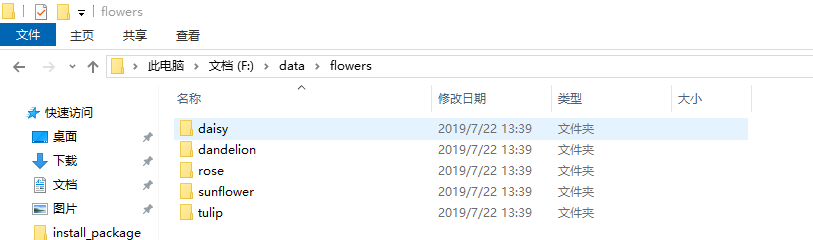
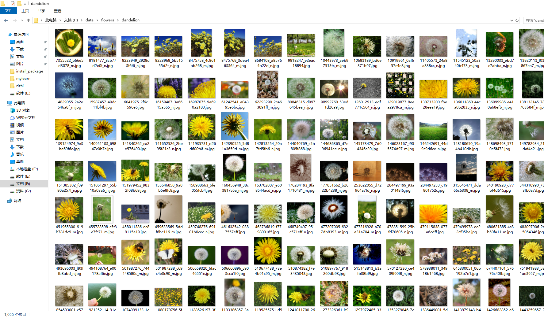
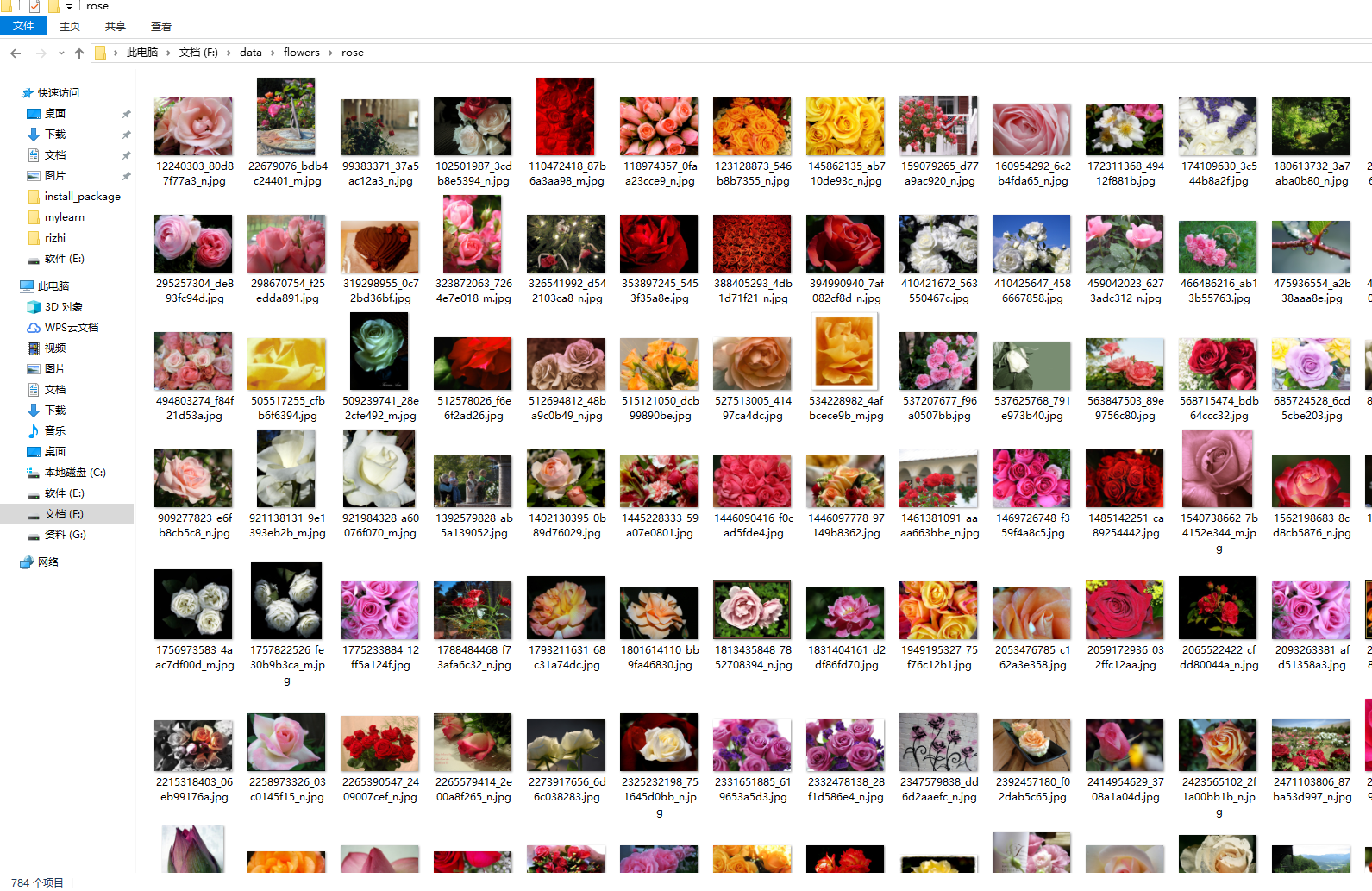
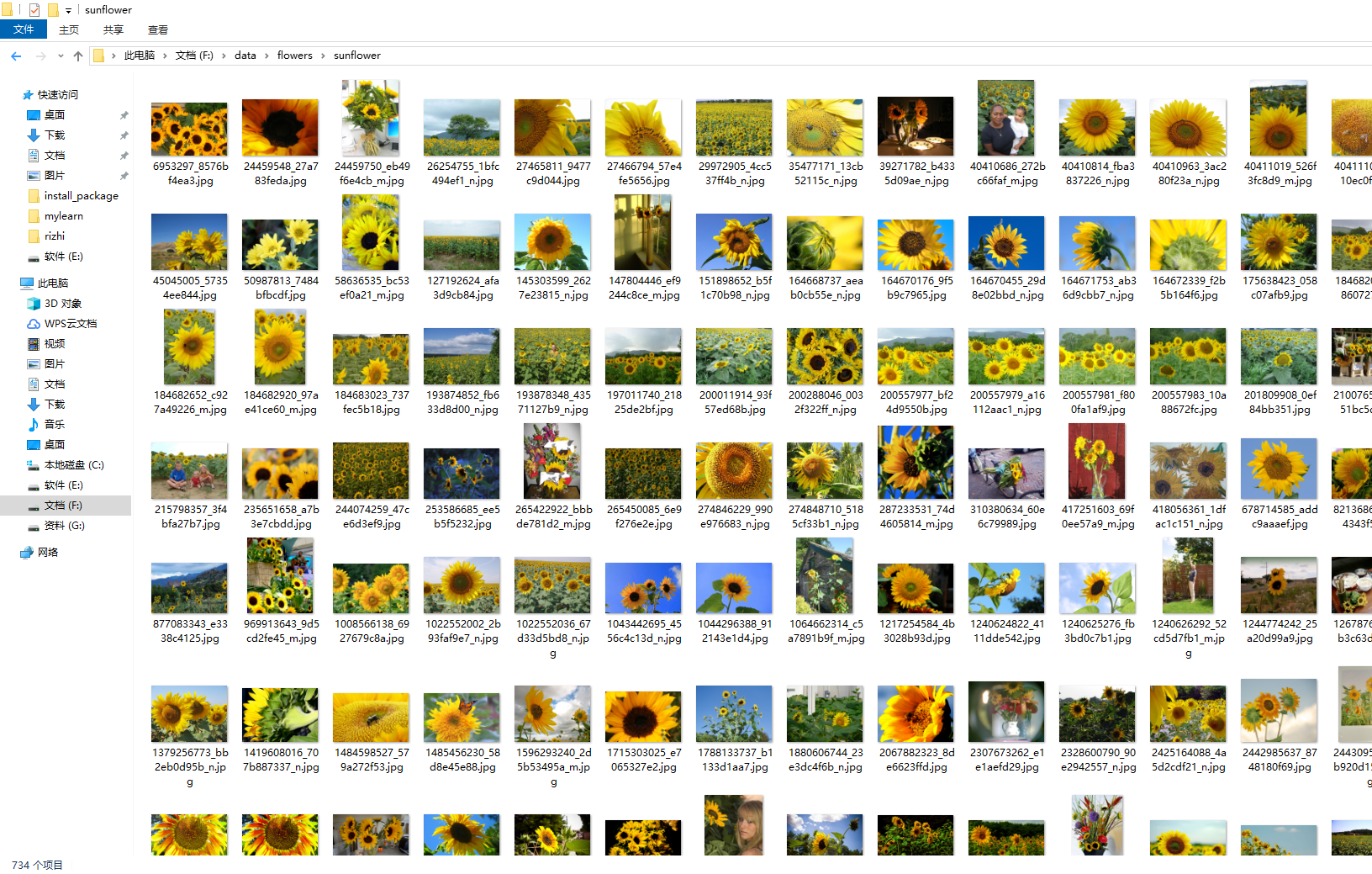
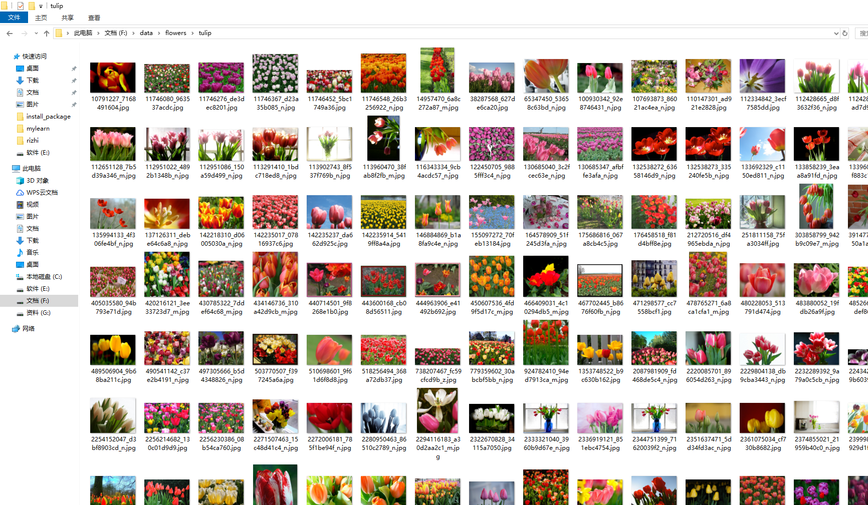
fileList = os.listdir("F:\\data\\flowers")
trainDataList = []
trianLabel = []
testDataList = []
testLabel = []

#读取每一种花的文件
for j in range(len(fileList)):
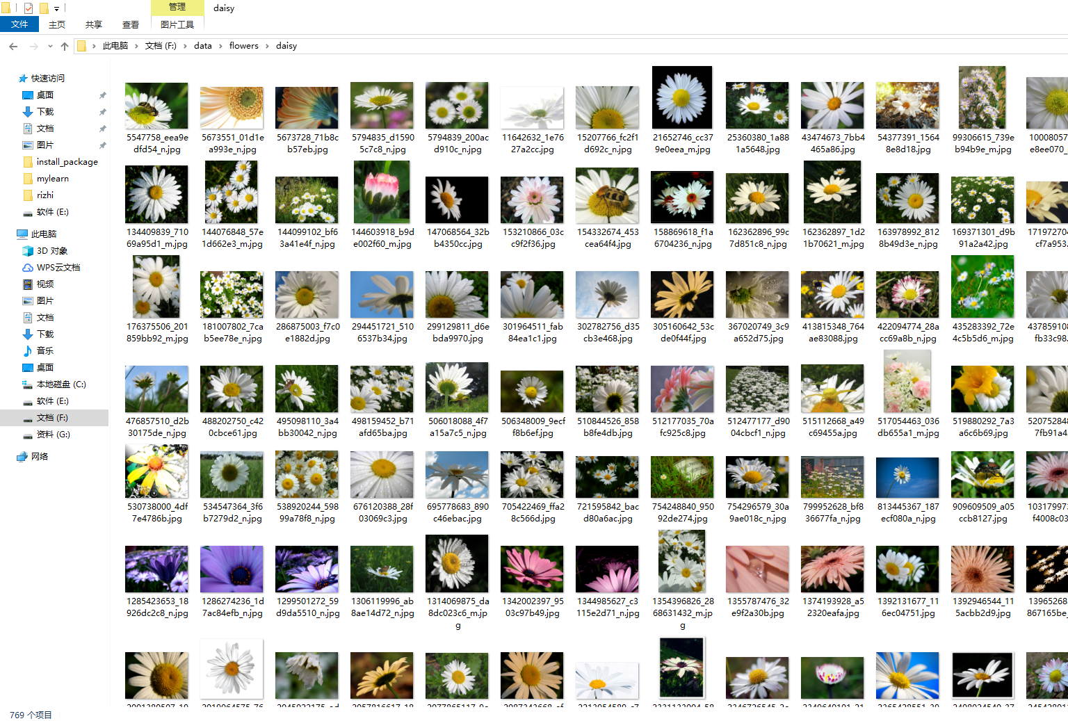
    data = os.listdir("F:\\data\\flowers\\"+fileList[j])
    #取每一种花四分之一的数据作为测试数据集
    testNum = int(len(data)*0.25)
    #把每种花的图片进行testNum次乱序处理
    while(testNum>0):
        np.random.shuffle(data)
        testNum -= 1
    #把每种花经过乱序后的四分之三当作训练集
    trainData = np.array(data[:-(int(len(data)*0.25))])
    #把每种花经过乱序后的四分之一当作测试集
    testData = np.array(data[-(int(len(data)*0.25)):])
    #从上面选出来的训练集中逐张读取出对应的图片
    for i in range(len(trainData)):
        #其中这些图片都要满足jpg格式的
        if(trainData[i][-3:]=="jpg"):
            #读取一张jpg图片
            image = io.imread("F:\\data\\flowers\\"+fileList[j]+"\\"+trainData[i])
            #把这张图片变成64*64大小的图片
            image=transform.resize(image,(64,64))
            #保存改变大小的图片到trainDataList列表
            trainDataList.append(image)
            #保存这张图片的标签到trianLabel列表
            trianLabel.append(int(j))
            #随机生成一个角度，这个角度的范围在顺时针90度和逆时针90度之间
            angle = np.random.randint(-90,90)
            #然后把上面那张64*64大小的图片随机旋转angle个角度
            image =transform.rotate(image, angle)
            #把旋转得到的新图片再变成64*64大小的，因为旋转会改变一张图片的大小
            image=transform.resize(image,(64,64))
            #把旋转后并且大小是64*64的图片保存到trainDataList列表
            trainDataList.append(image)
            #把旋转后并且大小是64*64的图片对应的标签保存到trianLabel列表
            trianLabel.append(int(j))
    #逐张读取每种花的测试图片
    for i in range(len(testData)):
        #选取的图片要满足jpg格式的
        if(testData[i][-3:]=="jpg"):
            #读取一张图片
            image = io.imread("F:\\data\\flowers\\"+fileList[j]+"\\"+testData[i])
            #改变这张图片的大小为64*64
            image=transform.resize(image,(64,64))
            #把改变后的图片保存到testDataList列表中
            testDataList.append(image)
            #把这张图片对应的标签保存到testLabel列表中
            testLabel.append(int(j))
print("图片数据读取完了...")

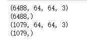
#打印训练集和测试数据集以及它们对应标签的规模
print(np.shape(trainDataList))
print(np.shape(trianLabel))
print(np.shape(testDataList))
print(np.shape(testLabel))

#保存训练集和测试数据集以及它们对应标签到磁盘
np.save("G:\\trainDataList",trainDataList)
np.save("G:\\trianLabel",trianLabel)
np.save("G:\\testDataList",testDataList)
np.save("G:\\testLabel",testLabel)
print("数据处理完了...")

import numpy as np
from keras.utils import to_categorical

#将训练数据集和测试数据集对应的标签转变为one-hot编码
trainLabel = np.load("G:\\trianLabel.npy")
testLabel = np.load("G:\\testLabel.npy")
trainLabel_encoded = to_categorical(trainLabel)
testLabel_encoded = to_categorical(testLabel)
np.save("G:\\trianLabel",trainLabel_encoded)
np.save("G:\\testLabel",testLabel_encoded)
print("转码类别写盘完了...")

import random
import numpy as np

trainDataList = np.load("G:\\trainDataList.npy")
trianLabel = np.load("G:\\trianLabel.npy")
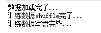
print("数据加载完了...")

trainIndex = [i for i in range(len(trianLabel))]
random.shuffle(trainIndex)
trainData = []
trainClass = []
for i in range(len(trainIndex)):
    trainData.append(trainDataList[trainIndex[i]])
    trainClass.append(trianLabel[trainIndex[i]])
print("训练数据shuffle完了...")

np.save("G:\\trainDataList",trainData)
np.save("G:\\trianLabel",trainClass)
print("训练数据写盘完毕...")

X = np.load("G:\\trainDataList.npy")
Y = np.load("G:\\trianLabel.npy")
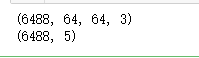
print(np.shape(X))
print(np.shape(Y))

import random
import numpy as np

testDataList = np.load("G:\\testDataList.npy")
testLabel = np.load("G:\\testLabel.npy")

testIndex = [i for i in range(len(testLabel))]
random.shuffle(testIndex)
testData = []
testClass = []
for i in range(len(testIndex)):
    testData.append(testDataList[testIndex[i]])
    testClass.append(testLabel[testIndex[i]])
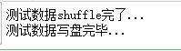
print("测试数据shuffle完了...")

np.save("G:\\testDataList",testData)
np.save("G:\\testLabel",testClass)
print("测试数据写盘完毕...")

X = np.load("G:\\testDataList.npy")
Y = np.load("G:\\testLabel.npy")
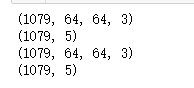
print(np.shape(X))
print(np.shape(Y))
print(np.shape(testData))
print(np.shape(testLabel))

import tensorflow as tf
from random import shuffle

INPUT_NODE = 64*64
OUT_NODE = 5
IMAGE_SIZE = 64
NUM_CHANNELS = 3
NUM_LABELS = 5

#第一层卷积层的尺寸和深度
CONV1_DEEP = 16
CONV1_SIZE = 5
#第二层卷积层的尺寸和深度
CONV2_DEEP = 32
CONV2_SIZE = 5
#全连接层的节点数
FC_SIZE = 512

def inference(input_tensor, train, regularizer):
    #卷积
    with tf.variable_scope('layer1-conv1'):
        conv1_weights = tf.Variable(tf.random_normal([CONV1_SIZE,CONV1_SIZE,NUM_CHANNELS,CONV1_DEEP],stddev=0.1),name='weight')
        tf.summary.histogram('convLayer1/weights1', conv1_weights)
        conv1_biases = tf.Variable(tf.Variable(tf.random_normal([CONV1_DEEP])),name="bias")
        tf.summary.histogram('convLayer1/bias1', conv1_biases)
        conv1 = tf.nn.conv2d(input_tensor,conv1_weights,strides=[1,1,1,1],padding='SAME')
        tf.summary.histogram('convLayer1/conv1', conv1)
        relu1 = tf.nn.relu(tf.nn.bias_add(conv1,conv1_biases))
        tf.summary.histogram('ConvLayer1/relu1', relu1)
    #池化
    with tf.variable_scope('layer2-pool1'):
        pool1 = tf.nn.max_pool(relu1,ksize=[1,2,2,1],strides=[1,2,2,1],padding='SAME')
        tf.summary.histogram('ConvLayer1/pool1', pool1)
    #卷积
    with tf.variable_scope('layer3-conv2'):
        conv2_weights = tf.Variable(tf.random_normal([CONV2_SIZE,CONV2_SIZE,CONV1_DEEP,CONV2_DEEP],stddev=0.1),name='weight')
        tf.summary.histogram('convLayer2/weights2', conv2_weights)
        conv2_biases = tf.Variable(tf.random_normal([CONV2_DEEP]),name="bias")
        tf.summary.histogram('convLayer2/bias2', conv2_biases)
        #卷积向前学习
        conv2 = tf.nn.conv2d(pool1,conv2_weights,strides=[1,1,1,1],padding='SAME')
        tf.summary.histogram('convLayer2/conv2', conv2)
        relu2 = tf.nn.relu(tf.nn.bias_add(conv2,conv2_biases))
        tf.summary.histogram('ConvLayer2/relu2', relu2)
    #池化
    with tf.variable_scope('layer4-pool2'):
        pool2 = tf.nn.max_pool(relu2,ksize=[1,2,2,1],strides=[1,2,2,1],padding='SAME')
        tf.summary.histogram('ConvLayer2/pool2', pool2)
    #变型
    pool_shape = pool2.get_shape().as_list()
    #计算最后一次池化后对象的体积（数据个数\节点数\像素个数）
    nodes = pool_shape[1]*pool_shape[2]*pool_shape[3]
    #根据上面的nodes再次把最后池化的结果pool2变为batch行nodes列的数据
    reshaped = tf.reshape(pool2,[-1,nodes])

    #全连接层
    with tf.variable_scope('layer5-fc1'):
        fc1_weights = tf.Variable(tf.random_normal([nodes,FC_SIZE],stddev=0.1),name='weight')
        if(regularizer != None):
            tf.add_to_collection('losses',tf.contrib.layers.l2_regularizer(0.03)(fc1_weights))
        fc1_biases = tf.Variable(tf.random_normal([FC_SIZE]),name="bias")
        #预测
        fc1 = tf.nn.relu(tf.matmul(reshaped,fc1_weights)+fc1_biases)
        if(train):
            fc1 = tf.nn.dropout(fc1,0.5)
    #全连接层
    with tf.variable_scope('layer6-fc2'):
        fc2_weights = tf.Variable(tf.random_normal([FC_SIZE,64],stddev=0.1),name="weight")
        if(regularizer != None):
            tf.add_to_collection('losses',tf.contrib.layers.l2_regularizer(0.03)(fc2_weights))
        fc2_biases = tf.Variable(tf.random_normal([64]),name="bias")
        #预测
        fc2 = tf.nn.relu(tf.matmul(fc1,fc2_weights)+fc2_biases)
        if(train):
            fc2 = tf.nn.dropout(fc2,0.5)
    #全连接层
    with tf.variable_scope('layer7-fc3'):
        fc3_weights = tf.Variable(tf.random_normal([64,NUM_LABELS],stddev=0.1),name="weight")
        if(regularizer != None):
            tf.add_to_collection('losses',tf.contrib.layers.l2_regularizer(0.03)(fc3_weights))
        fc3_biases = tf.Variable(tf.random_normal([NUM_LABELS]),name="bias")
        #预测
        logit = tf.matmul(fc2,fc3_weights)+fc3_biases
    return logit

import time
import keras
import numpy as np
from keras.utils import np_utils

X = np.load("G:\\trainDataList.npy")
Y = np.load("G:\\trianLabel.npy")
print(np.shape(X))
print(np.shape(Y))
print(np.shape(testData))
print(np.shape(testLabel))

batch_size = 10
n_classes=5
epochs=16#循环次数
learning_rate=1e-4
batch_num=int(np.shape(X)[0]/batch_size)
dropout=0.75

x=tf.placeholder(tf.float32,[None,64,64,3])
y=tf.placeholder(tf.float32,[None,n_classes])
# keep_prob = tf.placeholder(tf.float32)
#加载测试数据集
test_X = np.load("G:\\testDataList.npy")
test_Y = np.load("G:\\testLabel.npy")
back = 64
ro = int(len(test_X)/back)

#调用神经网络方法
pred=inference(x,1,"regularizer")
cost=tf.reduce_mean(tf.nn.softmax_cross_entropy_with_logits(logits=pred,labels=y))

# 三种优化方法选择一个就可以
optimizer=tf.train.AdamOptimizer(1e-4).minimize(cost)
# train_step = tf.train.GradientDescentOptimizer(0.001).minimize(cost)
# train_step = tf.train.MomentumOptimizer(0.001,0.9).minimize(cost)

#将预测label与真实比较
correct_pred=tf.equal(tf.argmax(pred,1),tf.argmax(y,1))
#计算准确率
accuracy=tf.reduce_mean(tf.cast(correct_pred,tf.float32))
merged=tf.summary.merge_all()
#将tensorflow变量实例化
init=tf.global_variables_initializer()
start_time = time.time()

with tf.Session() as sess:
    sess.run(init)
    #保存tensorflow参数可视化文件
    writer=tf.summary.FileWriter('F:/Flower_graph', sess.graph)
    for i in range(epochs):
        for j in range(batch_num):
            offset = (j * batch_size) % (Y.shape[0] - batch_size)
            # 准备数据
            batch_data = X[offset:(offset + batch_size), :]
            batch_labels = Y[offset:(offset + batch_size), :]
            sess.run(optimizer, feed_dict={x:batch_data,y:batch_labels})
            result=sess.run(merged, feed_dict={x:batch_data,y:batch_labels})
        writer.add_summary(result, i)
        loss,acc = sess.run([cost,accuracy],feed_dict={x:batch_data,y:batch_labels})
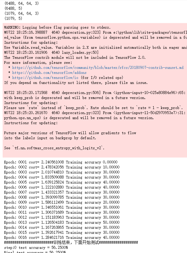
        print("Epoch:", '%04d' % (i+1),"cost=", "{:.9f}".format(loss),"Training accuracy","{:.5f}".format(acc*100))
    writer.close()
    print("########################训练结束，下面开始测试###################")
    for i in range(ro):
        s = i*back
        e = s+back
        test_accuracy = sess.run(accuracy,feed_dict={x:test_X[s:e],y:test_Y[s:e]})
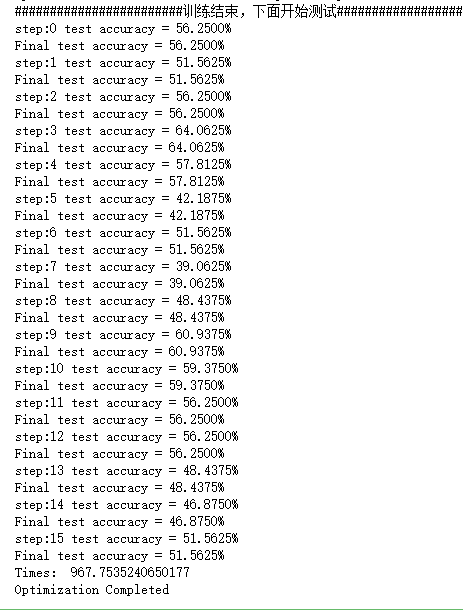
        print("step:%d test accuracy = %.4f%%" % (i,test_accuracy*100))
    print("Final test accuracy = %.4f%%" % (test_accuracy*100))

end_time = time.time()
print('Times：',(end_time-start_time))
print('Optimization Completed')