[论文分享] DHP: Differentiable Meta Pruning via HyperNetworks

[论文分享] DHP: Differentiable Meta Pruning via HyperNetworks

---

authors: Yawei Li1, Shuhang Gu, etc.

comments: ECCV2020

cite: [2003.13683] DHP: Differentiable Meta Pruning via HyperNetworks (arxiv.org)

code: ofsoundof/dhp: This is the official implementation of "DHP: Differentiable Meta Pruning via HyperNetworks". (github.com) (official)

---

0、速览

研究现状和存在问题

目前 AutoML 和 neural architecture search(NAS) 在剪枝领域的应用异常火爆，但是作者指出目前的自动剪枝要么依赖于强化学习（reinforcement learning）要不依赖于进化算法（evolutionary algorithm）。这些算法不具有可微性，所以需要较长的搜索阶段才能收敛。

本文为了解决这个问题，提出了新的基于超网络的可微剪枝方法，用于自动进行网络剪枝。

具体做法：

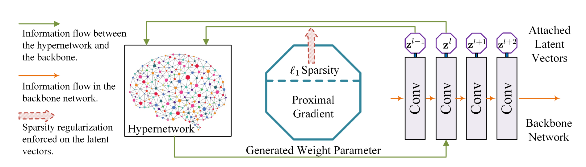
设计一个额外的超网络（hypernetwork），该超网络在初始化之后，训练后的输出作为骨干网（backbone network）的权值参数。

而骨干网络的输出（文中称为潜在向量，latent vector）在 一范数正则化和近端梯度求解后，得到稀疏潜在向量，超网络将前后两层 \(z^{l-1}、z^{l}\) 的稀疏潜在向量作为超网络的输入，训练之后的输出作为后一层 \(z^{l}\) 新的权值参数。相较于上次权值参数，相应的切片被去除，达到了网络剪枝的效果。

可微性来自为剪枝定制的超网络和近端梯度

---

1、介绍

With the advent of AutoML and neural architecture search (NAS) [63,8], a new trend of network pruning emerges, i.e. pruning with automatic algorithms and targeting distinguishing sub-architectures. Among them, reinforcement learning and evolutionary algorithm become the natural choice [19,40]. The core idea is to search a certain fine-grained layer-wise distinguishing configuration among the all of the possible choices (population in the terminology of evolutionary algorithm).After the searching stage, the candidate that optimizes the network prediction accuracy under constrained budgets is chosen.

随着AutoML和neural architecture search (NAS)的出现[63,8]，出现了一个新的网络剪枝趋势，即使用自动算法并针对不同的子架构进行剪枝。其中，强化学习和进化算法成为自然选择[19,40]。其核心思想是在所有可能的选择(进化算法术语中的种群)中搜索特定的细粒度分层区别配置。搜索阶段结束后，在预算受限的情况下，选择最优网络预测精度的候选算法。

However, the main concern of these algorithms is the convergence property.

这些算法关注点在于收敛性。强化学习存在着收敛困难的问题；进化算法无法训练整个种群直至收敛。

A promising solution to this problem is endowing the searching mechanism with differentiability or resorting to an approximately differentiable algorithm. This is due to the fact that differentiability has the potential to make the searching stage efficient。

一个有希望的解决方案就是赋予搜索机制可微性或近似可微，这会使得搜索阶段变得高效。

Actually, differentiability has facilitated a couple of machine learning approaches and the typical one among them is NAS. ... Differentiable architecture search (DARTS) reduces the insatiable consumption to tens of GPU hours ...

NAS 就是具有可微性的一种方案，但是早期过于耗时。后来的可微结构搜索（Differentiable architecture search）大大减小了GPU消耗时间。

Another noteworthy direction for automatic pruning is brought by MetaPruning [40] which introduces hypernetworks [13] into network compression .... ...

另一种解决思路是 MetaPruning，它将超网络引入到网络压缩中。超网络的输出被作为骨干网络的的参数；在训练过程中，梯度会被反向传播到超网络。这种方法属于meta learning 因为超网络中的参数是骨干网络参数的元数据（meta-data）。本文的方法属于MetaPruning。

... ...Each layer is endowed with a latent vector that controls the output channels of this layer. Since the layers in the network are connected, the latent vector also controls the input channel of the next layer. The hypernetwork takes as input the latent vectors of the current layer and previous layer that controls the output and input channels of the current layer respectively.

本文方法：骨干网络每一层被赋予一个潜在向量来控制这一层的输出通道。由于骨干网络中的每层是相互链接的，潜在向量也控制着下一层的输入通道。超网络以当前层和上一层的潜在向量作为输入，分别控制着当前层的输出通道和输入通道，输出结果被作为骨干网络当前层的新参数。

To achieve the effect of automatic pruning, ‘1sparsity regularizer is applied to the latent vectors. A pruned model is discovered by updating the latent vectors with proximal gradient. The searching stage stops when the compression ratio drops to the target level.

为了达到自动修剪的效果，对潜在向量应用了 \(l_1\) 稀疏正则化；利用近端梯度更新潜在向量，得到一个剪枝模型。当压缩比下降到目标水平后，搜索阶段停止，此时潜在向量已经被稀疏化了。

2、Methodology

2.1 超网络设计 Hypernetwork design

符号：标准（x）-> 标量；小写（z）-> 向量；大写（Z）-> 矩阵/高纬张量

超网络设计如上

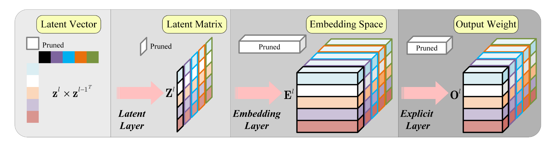
The hypernetwork consists of three layers. The latent layer takes as input the latent vectors and computes a latent matrix from them. The embedding layer projects the elements of the latent matrix to an embedding space. The last explicit layer converts the embedded vectors to the final output.

超网络一共有三层。第一层是潜在层（latent layers），负责将输入的潜在向量计算成潜在矩阵；第二层是嵌入层（embedding layer），负责将潜在矩阵的元素投射到嵌入空间（embedding space）；第三层是显示层，负责将嵌入向量转化成最终输出。

对于一个cnn，假设第 \(l\) 层的权值参数的维度为 \(n * c * w * h\)，这里的 \(n, c, w*h\) 分别表示输出通道，输入通道，卷积核尺寸。现在该层被赋予一个潜在向量 \(z^{l}\)，潜在向量的大小和该层的输出通道相同，同理上层 \(z^{l-1}\)。超参数网络以 \(z^l, z^{l-1}\) 为输入。第一层潜在向量的计算如下：

\[\mathbf { Z } ^ { l } = \mathbf { z } ^ { l } \cdot \mathbf { z } ^ { l - 1 ^ { T } } + \mathbf { B } _ { 0 } ^ { l }
\]

这里，\(\mathbf { Z } ^ { l } , \mathbf { B } _ { 0 } \in \mathbb { R } ^ { n \times c }\)。第二层公式：

\[\mathbf { E } _ { i , j } ^ { l } = \mathbf { Z } _ { i , j } ^ { l } \mathbf { w } _ { 1 } ^ { l } + \mathbf { b } _ { 1 } ^ { l } , i = 1 , \cdots , n , j = 1 , \cdots , c
\]

这里，\(\mathbf { E } _ { i , j } ^ { l } , \mathbf { w } _ { 1 } ^ { l } , \mathbf { b } _ { 1 } ^ { l } \in \mathbb { R } ^ { m }\)。\(\mathbf { E } _ { i , j } ^ { l } , \mathbf { w } _ { 1 } ^ { l } , \mathbf { b } _ { 1 } ^ { l }\) 聚合成3D张量，命名为 \(\mathbf { W } _ { 1 } ^ { l } , \mathbf { B } _ { 1 } ^ { l } , \mathbf { E } ^ { l } \in \mathbb { R } ^ { n \times c \times m }\)。第三次公式：

\[\mathbf { O } _ { i , j } ^ { l } = \mathbf { w } _ { 2 } ^ { l } \cdot \mathbf { E } _ { i , j } ^ { l } + \mathbf { b } _ { 2 } ^ { l } , i = 1 , \cdots , n , j = 1 , \cdots , c
\]

这里，\(\mathbf { O } _ { i , j } ^ { l } , \mathbf { b } _ { 2 } ^ { l } \in \mathbb { R } ^ { w h } , \mathbf { w } _ { 2 } ^ { l } \in \mathbb { R } ^ { w h \times m }\)。\(\mathbf { w } _ { 2 } ^ { l } , \mathbf { b } _ { 2 } ^ { l } , \text { and } \mathbf { O } _ { i , j } ^ { l }\)聚合成高维张量，\(\mathbf { W } _ { 2 } ^ { l } \in \mathbb { R } ^ { n \times c \times w h \times m }\)，\(\mathbf { B } _ { 2 } ^ { l } , \mathbf { O } ^ { l } \in\mathbb { R } ^ { n \times c \times w h }\)。抽象整合后：

\[\mathbf { O } ^ { l } = h \left( \mathbf { z } ^ { l } , \mathbf { z } ^ { l - 1 } ; \mathbf { W } ^ { l } , \mathbf { B } ^ { l } \right)
\]

此时，超网络的输出 \(O^{l}\) 被用作骨干网络第 \(l\) 层的权值参数。

The output \(O^l\) covariant with the input latent vector because pruning an element in the latent vector removes the corresponding slice of the output \(O^l\)

2.2 稀疏正则化和近端梯度 Sparsity regularization and proximal gradient

The core of differentiability comes with not only the specifically designed hypernetwork but also the mechanism used to search the the potential candidate. To achieve that, we enforce sparsity constraints to the latent vectors.

可微性的核心不仅存在于特别设计的超网络，而且在于用于搜索潜在候选人的机制。为了实现这一点，我们对潜在向量实施稀疏性约束。

假设上文提到的CNN的损失函数如下：

\[\min _ { \mathbf { W } , \mathbf { B } , \mathbf { z } } \mathcal { L } ( \mathbf { y } , f ( \mathbf { x } ; h ( \mathbf { z } ; \mathbf { W } , \mathbf { B } ) ) ) + \gamma \mathcal { D } ( \mathbf { W } ) + \gamma \mathcal { D } ( \mathbf { B } ) + \lambda \mathcal { R } ( \mathbf { z } )
\]

这里 \(\mathcal { L } ( \cdot , \cdot ) , \mathcal { D } ( \cdot ) , \text { and } \mathcal { R } ( \cdot )\) 分别是视觉任务的损失函数，权值衰减项损失函数，和稀疏正则化损失函数。\(\gamma， \lambda\) 是正则化因子。假设稀疏正则化采用的 \(l_1\) 正则化：\(\mathcal { R } ( \mathbf { z } ) = \sum _ { l = 1 } ^ { L } \left\| \mathbf { z } ^ { l } \right\| _ { 1 }\)。

注释： \(l_1\) 正则化可以使得参数稀疏但是往往会带来不可微的问题

为了解决损失函数，超网络中的权值 \(W\) 和偏置 \(B\) 会通过SGD更新。SGD中的梯度来自骨干网络的反向传播。而不可微部分则使用近端梯度方法进行更新，公式如下：

\[\mathbf { z } [ k + 1 ] = \operatorname { prox } _ { \lambda \mu \mathcal { R } } ( \mathbf { z } [ k ] - \lambda \mu \nabla \mathcal { L } ( \mathbf { z } [ k ] ) )
\]

这里的 \(\mu\) 是近端梯度的步长，同时也将它设作为 SGD 的学习率。当稀疏正则化采用的是 \(l_1\)，此时这个近端梯度有解析解：

\[\mathbf { z } [ k + 1 ] = \operatorname { sgn } ( \mathbf { z } [ k + \Delta ] ) [ | \mathbf { z } [ k + \Delta ] | - \lambda \mu ] _ { + }
\]

这里其实就是软阈值法计算。

因此，潜在向量会先得到 \(W, B\) 的 SGD 更新，然后近端算子更新。由于SGD更新和近端算子都有封闭解，所以可以认为整个解是近似可微的，这保证了算法与强化学习、进化算法相比是快速收敛。

2.3 网络剪枝 Network pruning

这块再看看再写

2.4 潜在向量共享 Latent vector sharing

... ... the residual blocks are interconnected with each other in the way that their input and output dimensions are related. Therefore, the skip connections are notoriously tricky to deal with.

由于 ResNet、MobileNetV2、SRResNet、EDSR 等残差网络存在 skip 连接，残差块之间以输入输出维度相关的方式相互连接。因此，处理跳跃连接十分棘手。

But back to the design of the proposed hypernetwork, a quite simple and straightforward solution to this problem is to let the hypernetworks of the correlated layers share the same latent vector. Note that the weight and bias parameters of the hypernetworks are not shared.

但是在超网络的设计中，这个问题的一个相当简单和直接的解决方案是让相关层的超网络共享相同的潜在向量。这里超网络的权值和偏差参数是不共享的。

Thus, sharing latent vectors does not force the the correlated layers to be identical. By automatically pruning the single latent vector, all of the relevant layers are pruned together.

因此，共享潜在向量并不强迫相关层是相同的。通过自动修剪单个潜在向量，所有相关的层被一起修剪。

2.5 收敛性的讨论 Discussion on the convergence property

讨论中作者指出几点：

Compared with reinforcement learning and evolutionary algorithm, proximal gradient may not be the optimal solution for some problems.

1. 和强化学习和进化算法相比，近端梯度可能不是某些问题的最优解

But as found by previous works [41,40], automatic network pruning serves as an implicit searching method for the channel configuration of a network.

1. 根据他人研究，自动网络剪枝是一种关于网络通道配置的隐式搜索方式

The important factor is the number of remaining channels of the convolutional layers in the network. Thus, it is relatively not important which filter is pruned as long as the number of pruned channels are the same.

1. 重要的是网络中卷积层剩余通道的数量，而不是哪个具体过滤器。

note：这个点我有些质疑，但作者没有给出进一步解释且我也没有证据反驳。先记着

2.6 Implementation consideration

超网络的紧凑表示：

将超网络中第二步公式 \(\mathbf { E } _ { i , j } ^ { l } = \mathbf { Z } _ { i , j } ^ { l } \mathbf { w } _ { 1 } ^ { l } + \mathbf { b } _ { 1 } ^ { l } , i = 1 , \cdots , n , j = 1 , \cdots , c\) 写成如下：

\[\mathbf { E } ^ { l } = \mathcal { U } ^ { 3 } \left( \mathbf { Z } ^ { l } \right) \circ \mathbf { W } _ { 1 } ^ { l } + \mathbf { B } _ { 1 } ^ { l }
\]

这里 \(\mathcal { U } ^ { 3 } \left( \mathbf { Z } ^ { l } \right) \in \mathbb { R } ^ { n \times c \times 1 }\) ，\(\mathcal { U } ^ { 3 } ( \cdot )\) 使得二维 \(Z^l\) 变成三维。超网络的第三步公式\(\mathbf { O } _ { i , j } ^ { l } = \mathbf { w } _ { 2 } ^ { l } \cdot \mathbf { E } _ { i , j } ^ { l } + \mathbf { b } _ { 2 } ^ { l } , i = 1 , \cdots , n , j = 1 , \cdots , c\) 写成如下：

\[\mathbf { O } ^ { l } = \mathbf { W } _ { 2 } ^ { l } * \mathbf { E } ^ { l } + \mathbf { B } _ { 2 } ^ { l }
\]

剪枝分析

分析超网络的三层以及隐藏的潜在向量，可以直接了解骨干层是如何自动剪枝的。公式如下：

\[\begin{aligned} \overline { \mathbf { O } } ^ { l } & = \mathbf { W } _ { 2 } ^ { l } * \left[ \mathcal { U } ^ { 3 } \left( \left( \mathbf { m } ^ { l } \circ \overline { \mathbf { z } } ^ { l } \right) \cdot \left( \mathbf { m } ^ { l - 1 } \circ \overline { \mathbf { z } } ^ { l - 1 } \right) ^ { T } \right) \circ \mathbf { W } _ { 1 } ^ { l } \right] \\ & = \mathbf { W } _ { 2 } ^ { l } * \left[ \mathcal { U } ^ { 3 } \left( \mathbf { m } ^ { l } \cdot \mathbf { m } ^ { l - 1 ^ { T } } \right) \circ \mathcal { U } ^ { 3 } \left( \overline { \mathbf { z } } ^ { l } \cdot \overline { \mathbf { z } } ^ { l - 1 ^ { T } } \right) \circ \mathbf { W } _ { 1 } ^ { l } \right]\\ & = \mathcal { U } ^ { 3 } \left( \mathbf { m } ^ { l } \cdot \mathbf { m } ^ { l - 1 ^ { T } } \right) \circ \left[ \mathbf { W } _ { 2 } ^ { l } * \left( \mathcal { U } ^ { 3 } \left( \overline { \mathbf { z } } ^ { l } \cdot \overline { \mathbf { z } } ^ { l - 1 ^ { T } } \right) \circ \mathbf { W } _ { 1 } ^ { l } \right) \right]\end{aligned}
\]

如上公式所示，在潜在向量上应用掩码与在最终输出上应用掩码具有相同的效果。

3、实验结果 Experimental Results

省略一个常见的错误率/FLOPs压缩率/参数压缩率的图

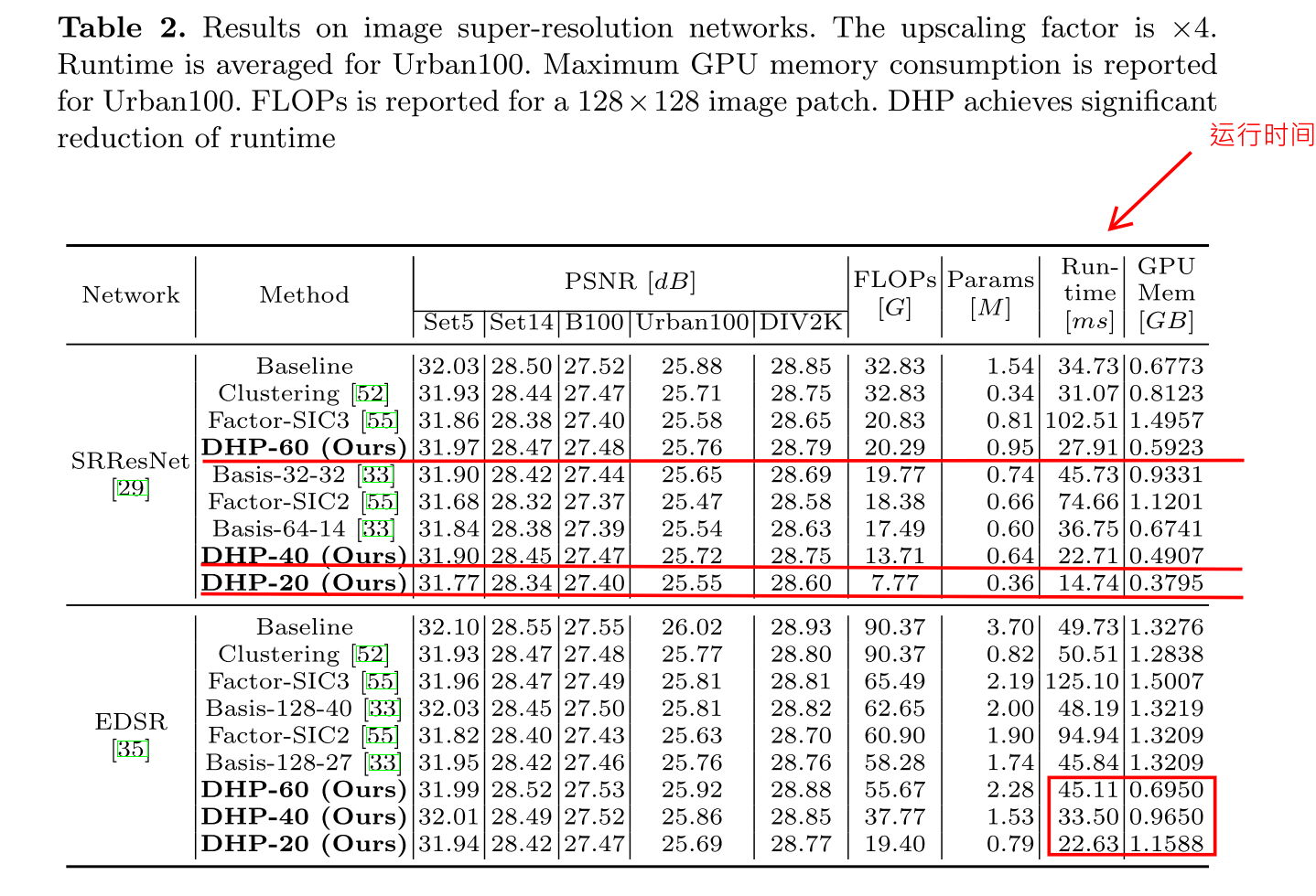
note：runtime 加速是真的不错