DSP using MATLAB 示例Example3.7

上代码：

x1 = rand(1,11); x2 = rand(1,11); n = 0:10;
alpha = 2; beta = 3; k = 0:500;
w = (pi/500)*k;              % [0,pi] axis divided into 501 points.

X1 = x1 * (exp(-j*pi/500)) .^ (n'*k);      % DTFT of x1
X2 = x2 * (exp(-j*pi/500)) .^ (n'*k);      % DTFT of x2

x = alpha * x1 + beta * x2;                % Linear combination of x1 & x2
X = x * (exp(-j*pi/500)) .^ (n'*k);        % DTFT of x

magX1 = abs(X1); angX1 = angle(X1); realX1 = real(X1); imagX1 = imag(X1);
magX2 = abs(X2); angX2 = angle(X2); realX2 = real(X2); imagX2 = imag(X2);
magX  = abs(X);  angX  = angle(X);  realX  = real(X);  imagX  = imag(X);

%verification
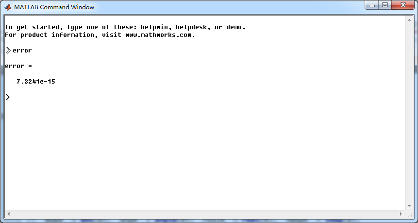
X_check = alpha*X1 + beta*X2;             % Linear combination of X1 & X2
error = max(abs(X-X_check));              % Difference

%% --------------------------------------------------------------
%%        START X1's  mag ang real imag
%% --------------------------------------------------------------
figure('NumberTitle', 'off', 'Name', 'X1 its Magnitude and Angle, Real and Imaginary Part');
set(gcf,'Color','white');
subplot(2,2,1); plot(w/pi,magX1); grid on;  % axis([-2,2,0,15]);
title('Magnitude Part');
xlabel('frequency in \pi units'); ylabel('Magnitude  |X1|');
subplot(2,2,3); plot(w/pi, angX1/pi); grid on;  % axis([-2,2,-1,1]);
title('Angle Part');
xlabel('frequency in \pi units'); ylabel('Radians/\pi');

subplot('2,2,2'); plot(w/pi, realX1); grid on;
title('Real Part');
xlabel('frequency in \pi units'); ylabel('Real');
subplot('2,2,4'); plot(w/pi, imagX1); grid on;
title('Imaginary Part');
xlabel('frequency in \pi units'); ylabel('Imaginary');
%% --------------------------------------------------------------
%%        END X1's  mag ang real imag
%% --------------------------------------------------------------

%% --------------------------------------------------------------
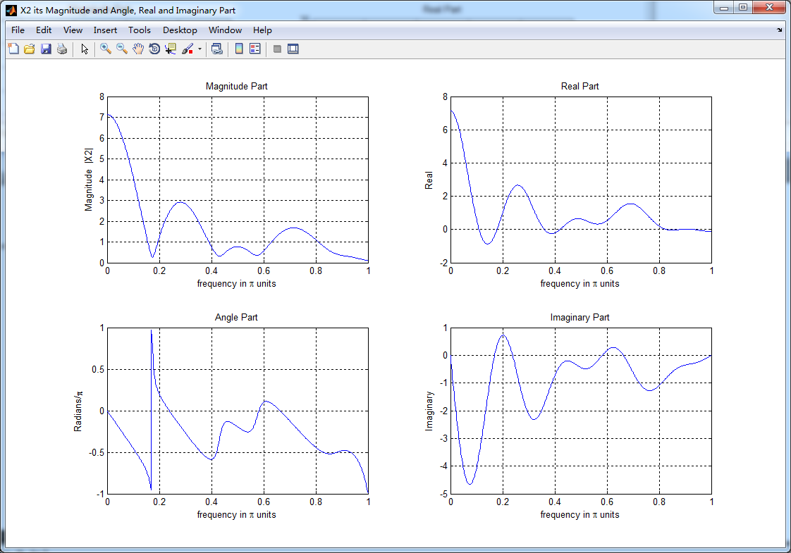
%%        START X2's  mag ang real imag
%% --------------------------------------------------------------
figure('NumberTitle', 'off', 'Name', 'X2 its Magnitude and Angle, Real and Imaginary Part');
set(gcf,'Color','white');
subplot(2,2,1); plot(w/pi,magX2); grid on;  % axis([-2,2,0,15]);
title('Magnitude Part');
xlabel('frequency in \pi units'); ylabel('Magnitude  |X2|');
subplot(2,2,3); plot(w/pi, angX2/pi); grid on;  % axis([-2,2,-1,1]);
title('Angle Part');
xlabel('frequency in \pi units'); ylabel('Radians/\pi');

subplot('2,2,2'); plot(w/pi, realX2); grid on;
title('Real Part');
xlabel('frequency in \pi units'); ylabel('Real');
subplot('2,2,4'); plot(w/pi, imagX2); grid on;
title('Imaginary Part');
xlabel('frequency in \pi units'); ylabel('Imaginary');
%% --------------------------------------------------------------
%%        END X2's  mag ang real imag
%% --------------------------------------------------------------

%% --------------------------------------------------------------
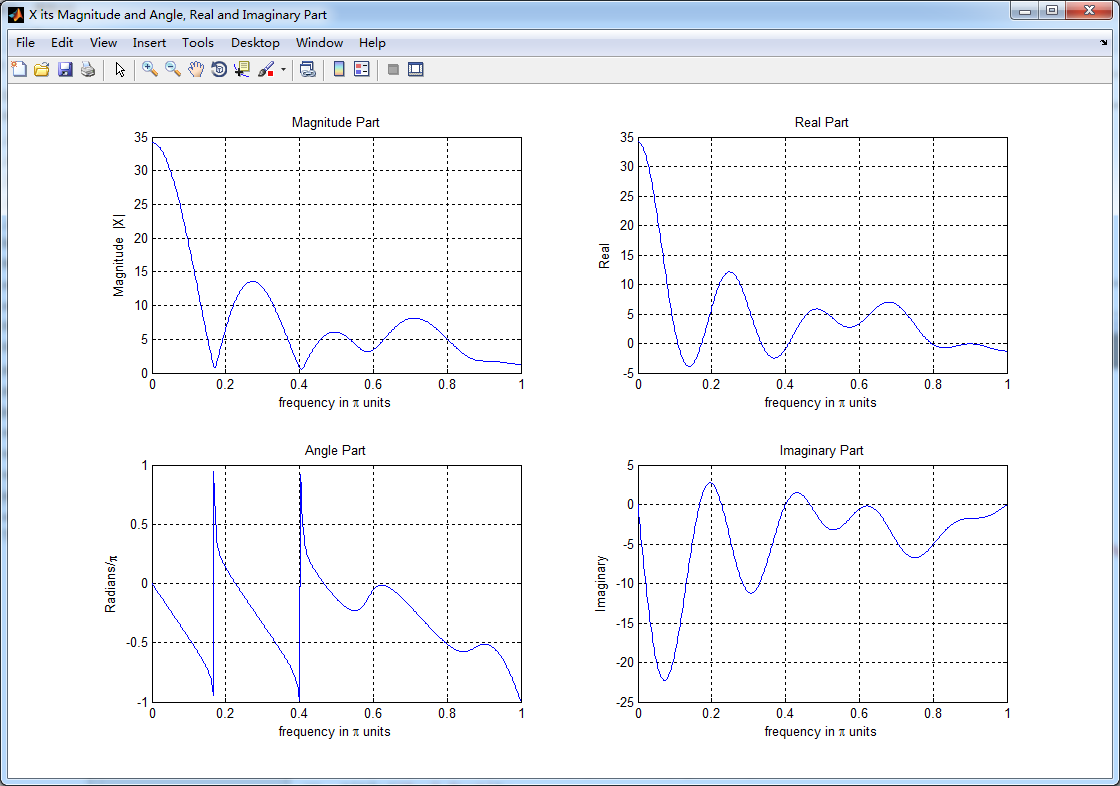
%%        START X's  mag ang real imag
%% --------------------------------------------------------------
figure('NumberTitle', 'off', 'Name', 'X its Magnitude and Angle, Real and Imaginary Part');
set(gcf,'Color','white');
subplot(2,2,1); plot(w/pi,magX); grid on;  % axis([-2,2,0,15]);
title('Magnitude Part');
xlabel('frequency in \pi units'); ylabel('Magnitude  |X|');
subplot(2,2,3); plot(w/pi, angX/pi); grid on;  % axis([-2,2,-1,1]);
title('Angle Part');
xlabel('frequency in \pi units'); ylabel('Radians/\pi');

subplot('2,2,2'); plot(w/pi, realX); grid on;
title('Real Part');
xlabel('frequency in \pi units'); ylabel('Real');
subplot('2,2,4'); plot(w/pi, imagX); grid on;
title('Imaginary Part');
xlabel('frequency in \pi units'); ylabel('Imaginary');

%% --------------------------------------------------------------
%%        END X's  mag ang real imag
%% --------------------------------------------------------------

结果: