DSP using MATLAB 示例 Example3.12

用到的性质

代码：

n = -5:10; x = sin(pi*n/2);
k = -100:100; w = (pi/100)*k;                 % freqency between -pi and +pi  ,   [0,pi] axis divided into 101 points.
X = x * (exp(-j*pi/100)) .^ (n'*k);           % DTFT of x

% signal decomposition
[xe,xo,m] = evenodd(x,n);                     % even and odd parts
XE = xe * (exp(-j*pi/100)) .^ (m'*k);         % DTFT of xe
XO = xo * (exp(-j*pi/100)) .^ (m'*k);         % DTFT of xo 

magXE = abs(XE); angXE = angle(XE); realXE = real(XE); imagXE = imag(XE);
magXO = abs(XO); angXO = angle(XO); realXO = real(XO); imagXO = imag(XO);
magX  = abs(X);  angX  = angle(X);  realX  = real(X);  imagX  = imag(X);

%verification
XR = real(X);                                  % real part of X
error1 = max(abs(XE-XR));                      % Difference
XI = imag(X);                                  % imag part of X
error2 = max(abs(XO-j*XI));                    % Difference

figure('NumberTitle', 'off', 'Name', 'x sequence')
set(gcf,'Color','white');
stem(n,x); title('x sequence'); xlabel('n'); ylabel('x(n)'); grid on;

figure('NumberTitle', 'off', 'Name', 'xe & xo sequence')
set(gcf,'Color','white');
subplot(2,1,1); stem(m,xe); title('xe sequence ');   xlabel('m'); ylabel('xe(m)'); grid on;
subplot(2,1,2); stem(m,xo); title('xo sequence ');   xlabel('m'); ylabel('xo(m)'); grid on;

%% --------------------------------------------------------------------
%%              START X's  mag ang real imag
%% --------------------------------------------------------------------
figure('NumberTitle', 'off', 'Name', 'X its Magnitude and Angle, Real and Imaginary Part');
set(gcf,'Color','white');
subplot(2,2,1); plot(w/pi,magX); grid on;  axis([-1,1,0,9]);
title('Magnitude Part');
xlabel('frequency in \pi units'); ylabel('Magnitude  |X|');
subplot(2,2,3); plot(w/pi, angX/pi); grid on;  axis([-1,1,-1,1]);
title('Angle Part');
xlabel('frequency in \pi units'); ylabel('Radians/\pi');

subplot('2,2,2'); plot(w/pi, realX); grid on;
title('Real Part');
xlabel('frequency in \pi units'); ylabel('Real');
subplot('2,2,4'); plot(w/pi, imagX); grid on;
title('Imaginary Part');
xlabel('frequency in \pi units'); ylabel('Imaginary');
%% -------------------------------------------------------------------
%%             END X's  mag ang real imag
%% -------------------------------------------------------------------

%% --------------------------------------------------------------
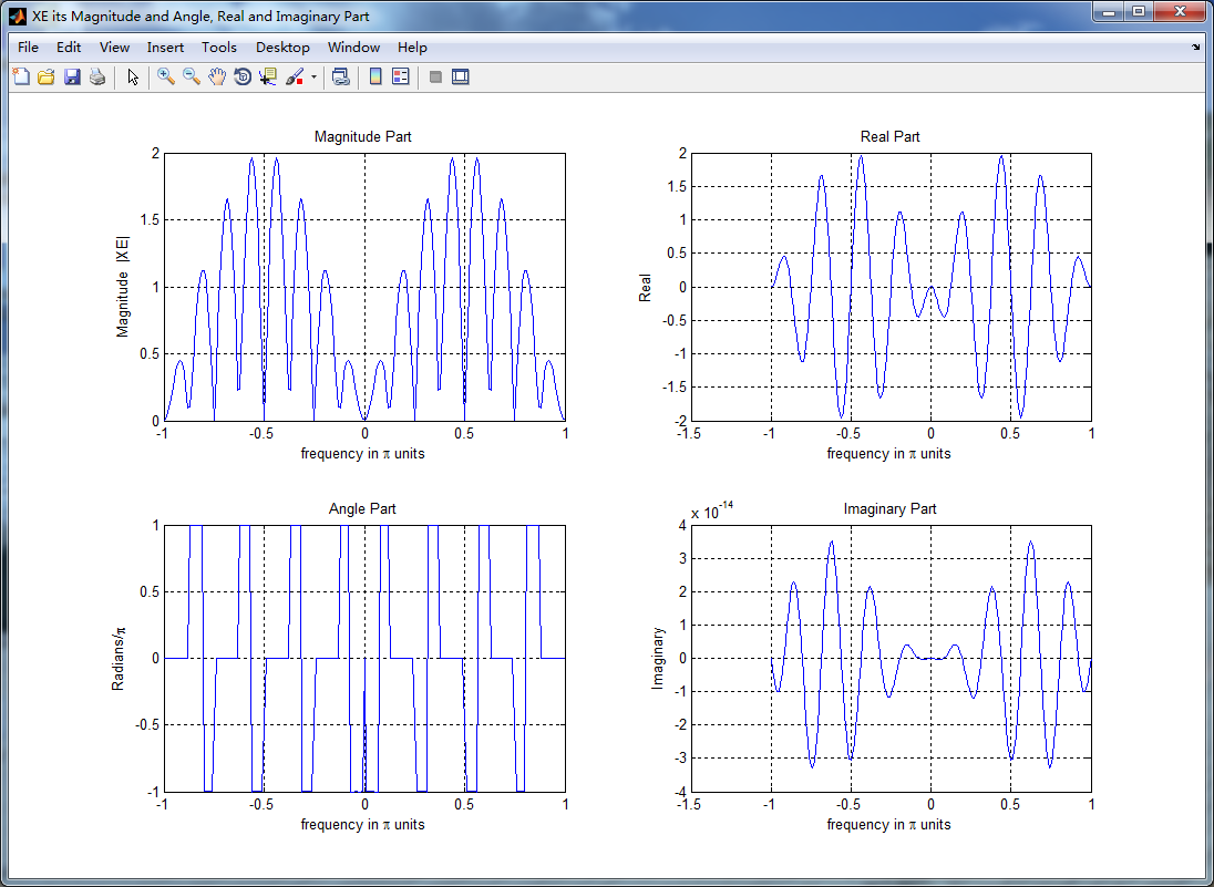
%%           START XE's  mag ang real imag
%% --------------------------------------------------------------
figure('NumberTitle', 'off', 'Name', 'XE its Magnitude and Angle, Real and Imaginary Part');
set(gcf,'Color','white');
subplot(2,2,1); plot(w/pi,magXE); grid on;  axis([-1,1,0,2]);
title('Magnitude Part');
xlabel('frequency in \pi units'); ylabel('Magnitude  |XE|');
subplot(2,2,3); plot(w/pi, angXE/pi); grid on;  axis([-1,1,-1,1]);
title('Angle Part');
xlabel('frequency in \pi units'); ylabel('Radians/\pi');

subplot('2,2,2'); plot(w/pi, realXE); grid on;
title('Real Part');
xlabel('frequency in \pi units'); ylabel('Real');
subplot('2,2,4'); plot(w/pi, imagXE); grid on;
title('Imaginary Part');
xlabel('frequency in \pi units'); ylabel('Imaginary');

%% --------------------------------------------------------------
%%             END XE's  mag ang real imag
%% --------------------------------------------------------------

%% --------------------------------------------------------------
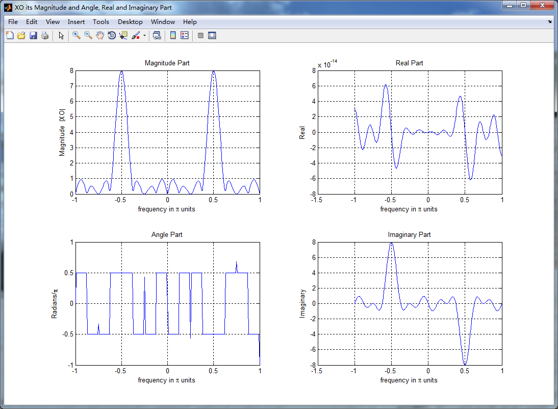
%%           START XO's  mag ang real imag
%% --------------------------------------------------------------
figure('NumberTitle', 'off', 'Name', 'XO its Magnitude and Angle, Real and Imaginary Part');
set(gcf,'Color','white');
subplot(2,2,1); plot(w/pi,magXO); grid on;  axis([-1,1,0,8]);
title('Magnitude Part');
xlabel('frequency in \pi units'); ylabel('Magnitude  |XO|');
subplot(2,2,3); plot(w/pi, angXO/pi); grid on;  axis([-1,1,-1,1]);
title('Angle Part');
xlabel('frequency in \pi units'); ylabel('Radians/\pi');

subplot('2,2,2'); plot(w/pi, realXO); grid on;
title('Real Part');
xlabel('frequency in \pi units'); ylabel('Real');
subplot('2,2,4'); plot(w/pi, imagXO); grid on;
title('Imaginary Part');
xlabel('frequency in \pi units'); ylabel('Imaginary');

%% --------------------------------------------------------------
%%             END XO's  mag ang real imag
%% --------------------------------------------------------------

%% ----------------------------------------------------------------
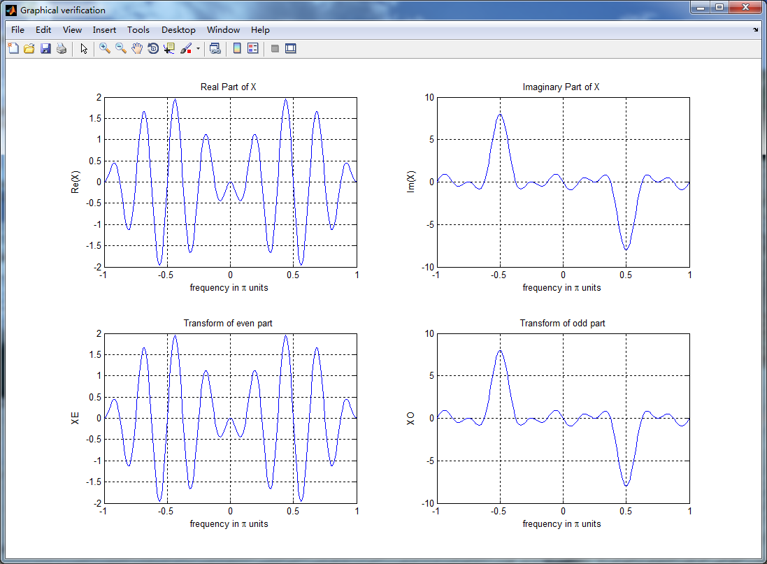
%%        START Graphical verification
%% ----------------------------------------------------------------
figure('NumberTitle', 'off', 'Name', 'Graphical verification');
set(gcf,'Color','white');
subplot(2,2,1); plot(w/pi,XR); grid on; axis([-1,1,-2,2]);
xlabel('frequency in \pi units'); ylabel('Re(X)'); title('Real Part of X ');
subplot(2,2,2); plot(w/pi,XI); grid on; axis([-1,1,-10,10]);
xlabel('frequency in \pi units'); ylabel('Im(X)'); title('Imaginary Part of X ');

subplot(2,2,3); plot(w/pi,realXE); grid on; axis([-1,1,-2,2]);
xlabel('frequency in \pi units'); ylabel('XE'); title('Transform of even part ');
subplot(2,2,4); plot(w/pi,imagXO); grid on; axis([-1,1,-10,10]);
xlabel('frequency in \pi units'); ylabel('XO'); title('Transform of odd part');

%% ----------------------------------------------------------------
%%        END Graphical verification
%% ----------------------------------------------------------------

　　运行结果：