下篇 | 使用 🤗 Transformers 进行概率时间序列预测

在《使用 Transformers 进行概率时间序列预测》的第一部分里，我们为大家介绍了传统时间序列预测和基于 Transformers 的方法，也一步步准备好了训练所需的数据集并定义了环境、模型、转换和 InstanceSplitter。本篇内容将包含从数据加载器，到前向传播、训练、推理和展望未来发展等精彩内容。

创建 PyTorch 数据加载器

有了数据，下一步需要创建 PyTorch DataLoaders。它允许我们批量处理成对的 (输入, 输出) 数据，即 (past_values , future_values)。

from gluonts.itertools import Cyclic, IterableSlice, PseudoShuffled
from gluonts.torch.util import IterableDataset
from torch.utils.data import DataLoader

from typing import Iterable

def create_train_dataloader(
    config: PretrainedConfig,
    freq,
    data,
    batch_size: int,
    num_batches_per_epoch: int,
    shuffle_buffer_length: Optional[int] = None,
    **kwargs,
) -> Iterable:
    PREDICTION_INPUT_NAMES = [
        "static_categorical_features",
        "static_real_features",
        "past_time_features",
        "past_values",
        "past_observed_mask",
        "future_time_features",
        ]

    TRAINING_INPUT_NAMES = PREDICTION_INPUT_NAMES + [
        "future_values",
        "future_observed_mask",
        ]

    transformation = create_transformation(freq, config)
    transformed_data = transformation.apply(data, is_train=True)

    # we initialize a Training instance
    instance_splitter = create_instance_splitter(
        config, "train"
    ) + SelectFields(TRAINING_INPUT_NAMES)

    # the instance splitter will sample a window of
    # context length + lags + prediction length (from the 366 possible transformed time series)
    # randomly from within the target time series and return an iterator.
    training_instances = instance_splitter.apply(
        Cyclic(transformed_data)
        if shuffle_buffer_length is None
        else PseudoShuffled(
            Cyclic(transformed_data),
            shuffle_buffer_length=shuffle_buffer_length,
        )
    )

    # from the training instances iterator we now return a Dataloader which will
    # continue to sample random windows for as long as it is called
    # to return batch_size of the appropriate tensors ready for training!
    return IterableSlice(
        iter(
            DataLoader(
                IterableDataset(training_instances),
                batch_size=batch_size,
                **kwargs,
            )
        ),
        num_batches_per_epoch,
    )

def create_test_dataloader(
    config: PretrainedConfig,
    freq,
    data,
    batch_size: int,
    **kwargs,
):
    PREDICTION_INPUT_NAMES = [
        "static_categorical_features",
        "static_real_features",
        "past_time_features",
        "past_values",
        "past_observed_mask",
        "future_time_features",
        ]

    transformation = create_transformation(freq, config)
    transformed_data = transformation.apply(data, is_train=False)

    # we create a Test Instance splitter which will sample the very last
    # context window seen during training only for the encoder.
    instance_splitter = create_instance_splitter(
        config, "test"
    ) + SelectFields(PREDICTION_INPUT_NAMES)

    # we apply the transformations in test mode
    testing_instances = instance_splitter.apply(transformed_data, is_train=False)

    # This returns a Dataloader which will go over the dataset once.
    return DataLoader(IterableDataset(testing_instances), batch_size=batch_size, **kwargs)

train_dataloader = create_train_dataloader(
    config=config,
    freq=freq,
    data=train_dataset,
    batch_size=256,
    num_batches_per_epoch=100,
)

test_dataloader = create_test_dataloader(
    config=config,
    freq=freq,
    data=test_dataset,
    batch_size=64,
)

让我们检查第一批:

batch = next(iter(train_dataloader))
for k,v in batch.items():
  print(k,v.shape, v.type())

>>> static_categorical_features torch.Size([256, 1]) torch.LongTensor
    static_real_features torch.Size([256, 1]) torch.FloatTensor
    past_time_features torch.Size([256, 181, 2]) torch.FloatTensor
    past_values torch.Size([256, 181]) torch.FloatTensor
    past_observed_mask torch.Size([256, 181]) torch.FloatTensor
    future_time_features torch.Size([256, 24, 2]) torch.FloatTensor
    future_values torch.Size([256, 24]) torch.FloatTensor
    future_observed_mask torch.Size([256, 24]) torch.FloatTensor

可以看出，我们没有将 input_ids 和 attention_mask 提供给编码器 (训练 NLP 模型时也是这种情况)，而是提供 past_values，以及 past_observed_mask、past_time_features、static_categorical_features 和 static_real_features 几项数据。

解码器的输入包括 future_values、future_observed_mask 和 future_time_features。 future_values 可以看作等同于 NLP 训练中的 decoder_input_ids。

我们可以参考 Time Series Transformer 文档 以获得对它们中每一个的详细解释。

前向传播

让我们对刚刚创建的批次执行一次前向传播:

# perform forward pass
outputs = model(
    past_values=batch["past_values"],
    past_time_features=batch["past_time_features"],
    past_observed_mask=batch["past_observed_mask"],
    static_categorical_features=batch["static_categorical_features"],
    static_real_features=batch["static_real_features"],
    future_values=batch["future_values"],
    future_time_features=batch["future_time_features"],
    future_observed_mask=batch["future_observed_mask"],
    output_hidden_states=True
)

print("Loss:", outputs.loss.item())

>>> Loss: 9.141253471374512

目前，该模型返回了损失值。这是由于解码器会自动将 future_values 向右移动一个位置以获得标签。这允许计算预测结果和标签值之间的误差。

另请注意，解码器使用 Causal Mask 来避免预测未来，因为它需要预测的值在 future_values 张量中。

训练模型

是时候训练模型了！我们将使用标准的 PyTorch 训练循环。

这里我们用到了 Accelerate 库，它会自动将模型、优化器和数据加载器放置在适当的 device 上。

from accelerate import Accelerator
from torch.optim import Adam

accelerator = Accelerator()
device = accelerator.device

model.to(device)
optimizer = Adam(model.parameters(), lr=1e-3)

model, optimizer, train_dataloader = accelerator.prepare(
    model, optimizer, train_dataloader,
)

for epoch in range(40):
    model.train()
    for batch in train_dataloader:
        optimizer.zero_grad()
        outputs = model(
            static_categorical_features=batch["static_categorical_features"].to(device),
            static_real_features=batch["static_real_features"].to(device),
            past_time_features=batch["past_time_features"].to(device),
            past_values=batch["past_values"].to(device),
            future_time_features=batch["future_time_features"].to(device),
            future_values=batch["future_values"].to(device),
            past_observed_mask=batch["past_observed_mask"].to(device),
            future_observed_mask=batch["future_observed_mask"].to(device),
        )
        loss = outputs.loss

        # Backpropagation
        accelerator.backward(loss)
        optimizer.step()

        print(loss.item())

推理

在推理时，建议使用 generate() 方法进行自回归生成，类似于 NLP 模型。

预测的过程会从测试实例采样器中获得数据。采样器会将数据集的每个时间序列的最后 context_length 那么长时间的数据采样出来，然后输入模型。请注意，这里需要把提前已知的 future_time_features 传递给解码器。

该模型将从预测分布中自回归采样一定数量的值，并将它们传回解码器最终得到预测输出:

model.eval()

forecasts = []

for batch in test_dataloader:
    outputs = model.generate(
        static_categorical_features=batch["static_categorical_features"].to(device),
        static_real_features=batch["static_real_features"].to(device),
        past_time_features=batch["past_time_features"].to(device),
        past_values=batch["past_values"].to(device),
        future_time_features=batch["future_time_features"].to(device),
        past_observed_mask=batch["past_observed_mask"].to(device),
    )
    forecasts.append(outputs.sequences.cpu().numpy())

该模型输出一个表示结构的张量 (batch_size, number of samples, prediction length)。

下面的输出说明: 对于大小为 64 的批次中的每个示例，我们将获得接下来 24 个月内的 100 个可能的值:

forecasts[0].shape

>>> (64, 100, 24)

我们将垂直堆叠它们，以获得测试数据集中所有时间序列的预测:

forecasts = np.vstack(forecasts)
print(forecasts.shape)

>>> (366, 100, 24)

我们可以根据测试集中存在的样本值，根据真实情况评估生成的预测。这里我们使用数据集中的每个时间序列的 MASE 和 sMAPE 指标 (metrics) 来评估:

from evaluate import load
from gluonts.time_feature import get_seasonality

mase_metric = load("evaluate-metric/mase")
smape_metric = load("evaluate-metric/smape")

forecast_median = np.median(forecasts, 1)

mase_metrics = []
smape_metrics = []
for item_id, ts in enumerate(test_dataset):
    training_data = ts["target"][:-prediction_length]
    ground_truth = ts["target"][-prediction_length:]
    mase = mase_metric.compute(
        predictions=forecast_median[item_id],
        references=np.array(ground_truth),
        training=np.array(training_data),
        periodicity=get_seasonality(freq))
    mase_metrics.append(mase["mase"])

    smape = smape_metric.compute(
        predictions=forecast_median[item_id],
        references=np.array(ground_truth),
    )
    smape_metrics.append(smape["smape"])

print(f"MASE: {np.mean(mase_metrics)}")

>>> MASE: 1.361636922541396

print(f"sMAPE: {np.mean(smape_metrics)}")

>>> sMAPE: 0.17457818831512306

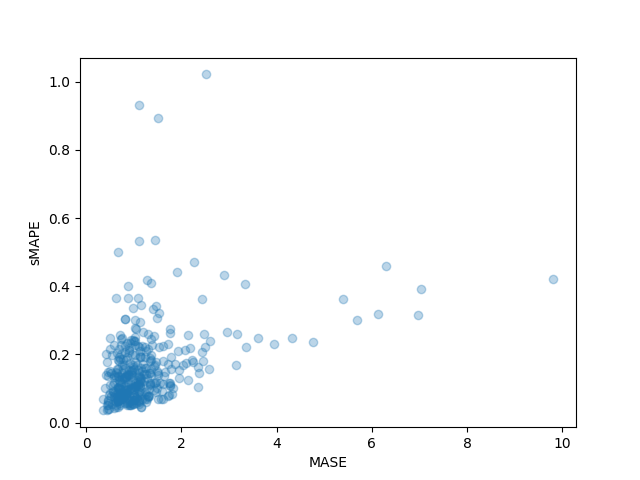
我们还可以单独绘制数据集中每个时间序列的结果指标，并观察到其中少数时间序列对最终测试指标的影响很大:

plt.scatter(mase_metrics, smape_metrics, alpha=0.3)
plt.xlabel("MASE")
plt.ylabel("sMAPE")
plt.show()

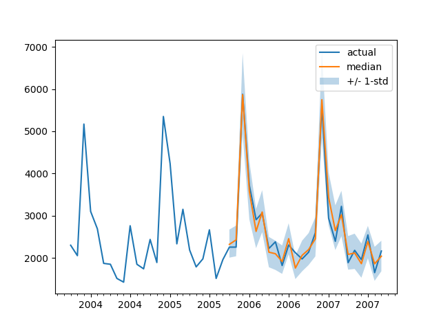
为了根据基本事实测试数据绘制任何时间序列的预测，我们定义了以下辅助绘图函数:

import matplotlib.dates as mdates

def plot(ts_index):
    fig, ax = plt.subplots()

    index = pd.period_range(
        start=test_dataset[ts_index][FieldName.START],
        periods=len(test_dataset[ts_index][FieldName.TARGET]),
        freq=freq,
    ).to_timestamp()

    # Major ticks every half year, minor ticks every month,
    ax.xaxis.set_major_locator(mdates.MonthLocator(bymonth=(1, 7)))
    ax.xaxis.set_minor_locator(mdates.MonthLocator())

    ax.plot(
        index[-2*prediction_length:],
        test_dataset[ts_index]["target"][-2*prediction_length:],
        label="actual",
    )

    plt.plot(
        index[-prediction_length:],
        np.median(forecasts[ts_index], axis=0),
        label="median",
    )

    plt.fill_between(
        index[-prediction_length:],
        forecasts[ts_index].mean(0) - forecasts[ts_index].std(axis=0),
        forecasts[ts_index].mean(0) + forecasts[ts_index].std(axis=0),
        alpha=0.3,
        interpolate=True,
        label="+/- 1-std",
    )
    plt.legend()
    plt.show()

例如:

plot(334)

我们如何与其他模型进行比较？ Monash Time Series Repository 有一个测试集 MASE 指标的比较表。我们可以将自己的结果添加到其中作比较:

Dataset	SES	Theta	TBATS	ETS	(DHR-)ARIMA	PR	CatBoost	FFNN	DeepAR	N-BEATS	WaveNet	Transformer (Our)
Tourism Monthly	3.306	1.649	1.751	1.526	1.589	1.678	1.699	1.582	1.409	1.574	1.482	1.361

请注意，我们的模型击败了所有已知的其他模型 (另请参见相应 论文 中的表 2) ，并且我们没有做任何超参数优化。我们仅仅花了 40 个完整训练调参周期来训练 Transformer。

当然，我们应该谦虚。从历史发展的角度来看，现在认为神经网络解决时间序列预测问题是正途，就好比当年的论文得出了 “你需要的就是 XGBoost” 的结论。我们只是很好奇，想看看神经网络能带我们走多远，以及 Transformer 是否会在这个领域发挥作用。这个特定的数据集似乎表明它绝对值得探索。

下一步

我们鼓励读者尝试我们的 Jupyter Notebook 和来自 Hugging Face Hub 的其他时间序列数据集，并替换适当的频率和预测长度参数。对于您的数据集，需要将它们转换为 GluonTS 的惯用格式，在他们的 文档 里有非常清晰的说明。我们还准备了一个示例 Notebook，向您展示如何将数据集转换为 Hugging Face 数据集格式。

正如时间序列研究人员所知，人们对“将基于 Transformer 的模型应用于时间序列”问题很感兴趣。传统 vanilla Transformer 只是众多基于注意力 (Attention) 的模型之一，因此需要向库中补充更多模型。

目前没有什么能妨碍我们继续探索对多变量时间序列 (multivariate time series) 进行建模，但是为此需要使用多变量分布头 (multivariate distribution head) 来实例化模型。目前已经支持了对角独立分布 (diagonal independent distributions)，后续会增加其他多元分布支持。请继续关注未来的博客文章以及其中的教程。

路线图上的另一件事是时间序列分类。这需要将带有分类头的时间序列模型添加到库中，例如用于异常检测这类任务。

当前的模型会假设日期时间和时间序列值都存在，但在现实中这可能不能完全满足。例如 WOODS 给出的神经科学数据集。因此，我们还需要对当前模型进行泛化，使某些输入在整个流水线中可选。

最后，NLP/CV 领域从大型预训练模型 中获益匪浅，但据我们所知，时间序列领域并非如此。基于 Transformer 的模型似乎是这一研究方向的必然之选，我们迫不及待地想看看研究人员和从业者会发现哪些突破！

---

英文原文: Probabilistic Time Series Forecasting with Transformers

译者、排版: zhongdongy (阿东)