Gradient Boosted Regression Trees 2

Regularization

GBRT provide three knobs to control overfitting: tree structure, shrinkage, and randomization.

Tree Structure

The depth of the individual trees is one aspect of model complexity. The depth of the trees basically control the degree of feature interactions that your model can fit. For example, if you want to capture the interaction between a feature latitude and a feature longitude your trees need a depth of at least two to capture this. Unfortunately, the degree of feature interactions is not known in advance but it is usually fine to assume that it is faily low -- in practise, a depth of 4-6 usually gives the best results. In scikit-learn you can constrain the depth of the trees using the max_depth argument.

Another way to control the depth of the trees is by enforcing a lower bound on the number of samples in a leaf: this will avoid inbalanced splits where a leaf is formed for just one extreme data point. In scikit-learn you can do this using the argument min_samples_leaf. This is effectively a means to introduce bias into your model with the hope to also reduce variance as shown in the example below:

def fmt_params(params):
    return ", ".join("{0}={1}".format(key, val) for key, val in params.iteritems())fig = plt.figure(figsize=(8, 5))ax = plt.gca()for params, (test_color, train_color) in [({}, ('#d7191c', '#2c7bb6')),
                                          ({'min_samples_leaf': 3},
                                           ('#fdae61', '#abd9e9'))]:
    est = GradientBoostingRegressor(n_estimators=n_estimators, max_depth=1, learning_rate=1.0)
    est.set_params(**params)
    est.fit(X_train, y_train)

    test_dev, ax = deviance_plot(est, X_test, y_test, ax=ax, label=fmt_params(params),
                                 train_color=train_color, test_color=test_color)
    ax.annotate('Higher bias', xy=(900, est.train_score_[899]), xycoords='data',
            xytext=(600, 0.3), textcoords='data',
            arrowprops=dict(arrowstyle="->", connectionstyle="arc"),
            )ax.annotate('Lower variance', xy=(900, test_dev[899]), xycoords='data',
            xytext=(600, 0.4), textcoords='data',
            arrowprops=dict(arrowstyle="->", connectionstyle="arc"),
            )plt.legend(loc='upper right')

Shrinkage

The most important regularization technique for GBRT is shrinkage: the idea is basically to do slow learning by shrinking the predictions of each individual tree by some small scalar, the learning_rate. By doing so the model has to re-enforce concepts. A lower learning_rate requires a higher number of n_estimatorsto get to the same level of training error -- so its trading runtime against accuracy.

fig = plt.figure(figsize=(8, 5))ax = plt.gca()for params, (test_color, train_color) in [({}, ('#d7191c', '#2c7bb6')),
                                          ({'learning_rate': 0.1},
                                           ('#fdae61', '#abd9e9'))]:
    est = GradientBoostingRegressor(n_estimators=n_estimators, max_depth=1, learning_rate=1.0)
    est.set_params(**params)
    est.fit(X_train, y_train)

    test_dev, ax = deviance_plot(est, X_test, y_test, ax=ax, label=fmt_params(params),
                                 train_color=train_color, test_color=test_color)
    ax.annotate('Requires more trees', xy=(200, est.train_score_[199]), xycoords='data',
            xytext=(300, 1.0), textcoords='data',
            arrowprops=dict(arrowstyle="->", connectionstyle="arc"),
            )ax.annotate('Lower test error', xy=(900, test_dev[899]), xycoords='data',
            xytext=(600, 0.5), textcoords='data',
            arrowprops=dict(arrowstyle="->", connectionstyle="arc"),
            )plt.legend(loc='upper right')

Stochastic Gradient Boosting

Similar to RandomForest, introducing randomization into the tree building process can lead to higher accuracy. Scikit-learn provides two ways to introduce randomization: a) subsampling the training set before growing each tree (subsample) and b) subsampling the features before finding the best split node (max_features). Experience showed that the latter works better if there is a sufficient large number of features (>30). One thing worth noting is that both options reduce runtime.

Below we show the effect of using subsample=0.5, ie. growing each tree on 50% of the training data, on our toy example:

fig = plt.figure(figsize=(8, 5))ax = plt.gca()for params, (test_color, train_color) in [({}, ('#d7191c', '#2c7bb6')),
                                          ({'learning_rate': 0.1, 'subsample': 0.5},
                                           ('#fdae61', '#abd9e9'))]:
    est = GradientBoostingRegressor(n_estimators=n_estimators, max_depth=1, learning_rate=1.0,
                                    random_state=1)
    est.set_params(**params)
    est.fit(X_train, y_train)
    test_dev, ax = deviance_plot(est, X_test, y_test, ax=ax, label=fmt_params(params),
                                 train_color=train_color, test_color=test_color)
    ax.annotate('Even lower test error', xy=(400, test_dev[399]), xycoords='data',
            xytext=(500, 0.5), textcoords='data',
            arrowprops=dict(arrowstyle="->", connectionstyle="arc"),
            )est = GradientBoostingRegressor(n_estimators=n_estimators, max_depth=1, learning_rate=1.0,
                                subsample=0.5)est.fit(X_train, y_train)test_dev, ax = deviance_plot(est, X_test, y_test, ax=ax, label=fmt_params({'subsample': 0.5}),
                             train_color='#abd9e9', test_color='#fdae61', alpha=0.5)ax.annotate('Subsample alone does poorly', xy=(300, test_dev[299]), xycoords='data',
            xytext=(250, 1.0), textcoords='data',
            arrowprops=dict(arrowstyle="->", connectionstyle="arc"),
            )plt.legend(loc='upper right', fontsize='small')

Hyperparameter tuning

We now have introduced a number of hyperparameters -- as usual in machine learning it is quite tedious to optimize them. Especially, since they interact with each other (learning_rate and n_estimators, learning_rate and subsample, max_depth and max_features).

We usually follow this recipe to tune the hyperparameters for a gradient boosting model:

Choose loss based on your problem at hand (ie. target metric)
Pick n_estimators as large as (computationally) possible (e.g. 3000).
Tune max_depth, learning_rate, min_samples_leaf, and max_features via grid search.
Increase n_estimators even more and tune learning_rate again holding the other parameters fixed.

Scikit-learn provides a convenient API for hyperparameter tuning and grid search:

from sklearn.grid_search import GridSearchCVparam_grid = {'learning_rate': [0.1, 0.05, 0.02, 0.01],
              'max_depth': [4, 6],
              'min_samples_leaf': [3, 5, 9, 17],
              # 'max_features': [1.0, 0.3, 0.1] ## not possible in our example (only 1 fx)
              }est = GradientBoostingRegressor(n_estimators=3000)# this may take some minutesgs_cv = GridSearchCV(est, param_grid, n_jobs=4).fit(X_train, y_train)# best hyperparameter settinggs_cv.best_params_

Out:{'learning_rate': 0.05, 'max_depth': 6, 'min_samples_leaf': 5}

Use-case: California Housing

This use-case study shows how to apply GBRT to a real-world dataset. The task is to predict the log median house value for census block groups in California. The dataset is based on the 1990 censues comprising roughly 20.000 groups. There are 8 features for each group including: median income, average house age, latitude, and longitude. To be consistent with [Hastie et al., The Elements of Statistical Learning, Ed2] we use Mean Absolute Error as our target metric and evaluate the results on an 80-20 train-test split.

import pandas as pdfrom sklearn.datasets.california_housing import fetch_california_housingcal_housing = fetch_california_housing()# split 80/20 train-testX_train, X_test, y_train, y_test = train_test_split(cal_housing.data,
                                                    np.log(cal_housing.target),
                                                    test_size=0.2,
                                                    random_state=1)names = cal_housing.feature_names

Some of the aspects that make this dataset challenging are: a) heterogenous features (different scales and distributions) and b) non-linear feature interactions (specifically latitude and longitude). Furthermore, the data contains some extreme values of the response (log median house value) -- such a dataset strongly benefits from robust regression techniques such as huberized loss functions.

Below you can see histograms for some of the features and the response. You can see that they are quite different: median income is left skewed, latitude and longitude are bi-modal, and log median house value is right skewed.

import pandas as pdX_df = pd.DataFrame(data=X_train, columns=names)X_df['LogMedHouseVal'] = y_train_ = X_df.hist(column=['Latitude', 'Longitude', 'MedInc', 'LogMedHouseVal'])


est = GradientBoostingRegressor(n_estimators=3000, max_depth=6, learning_rate=0.04,
                                loss='huber', random_state=0)est.fit(X_train, y_train)

GradientBoostingRegressor(alpha=0.9, init=None, learning_rate=0.04,
             loss='huber', max_depth=6, max_features=None,
             max_leaf_nodes=None, min_samples_leaf=1, min_samples_split=2,
             n_estimators=3000, random_state=0, subsample=1.0, verbose=0,
             warm_start=False)

from sklearn.metrics import mean_absolute_errormae = mean_absolute_error(y_test, est.predict(X_test))print('MAE: %.4f' % mae)

Feature importance

Often features do not contribute equally to predict the target response. When interpreting a model, the first question usually is: what are those important features and how do they contributing in predicting the target response?

A GBRT model derives this information from the fitted regression trees which intrinsically perform feature selection by choosing appropriate split points. You can access this information via the instance attribute est.feature_importances_.

# sort importancesindices = np.argsort(est.feature_importances_)# plot as bar chartplt.barh(np.arange(len(names)), est.feature_importances_[indices])plt.yticks(np.arange(len(names)) + 0.25, np.array(names)[indices])_ = plt.xlabel('Relative importance')

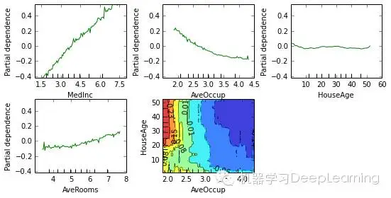
Partial dependence

Partial dependence plots show the dependence between the response and a set of features, marginalizing over the values of all other features. Intuitively, we can interpret the partial dependence as the expected response as a function of the features we conditioned on.

The plot below contains 4 one-way partial depencence plots (PDP) each showing the effect of an idividual feature on the repsonse. We can see that median incomeMedInc has a linear relationship with the log median house value. The contour plot shows a two-way PDP. Here we can see an interesting feature interaction. It seems that house age itself has hardly an effect on the response but when AveOccup is small it has an effect (the older the house the higher the price).

from sklearn.ensemble.partial_dependence import plot_partial_dependencefeatures = ['MedInc', 'AveOccup', 'HouseAge', 'AveRooms',
            ('AveOccup', 'HouseAge')]fig, axs = plot_partial_dependence(est, X_train, features,
                                   feature_names=names, figsize=(8, 6))

Scikit-learn provides a convenience function to create such plots: sklearn.ensemble.partial_dependence.plot_partial_dependence or a low-level function that you can use to create custom partial dependence plots (e.g. map overlays or 3d