吴恩达深度学习笔记（五） —— 优化算法：Mini-Batch GD、Momentum、RMSprop、Adam、学习率衰减

主要内容：

一.Mini-Batch Gradient descent

二.Momentum

四.RMSprop

五.Adam

六.优化算法性能比较

七.学习率衰减

一.Mini-Batch Gradient descent

1.一般地，有三种梯度下降算法：

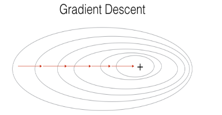
1）（Batch ）Gradient Descent，即我们平常所用的。它在每次求梯度的时候用上所有数据集，此种方式适合用在数据集规模不大的情况下。

X = data_input

Y = labels

parameters = initialize_parameters(layers_dims)

for i in range(0, num_iterations):

    # Forward propagation

    a, caches = forward_propagation(X, parameters)

    # Compute cost.

    cost = compute_cost(a, Y)

    # Backward propagation.

    grads = backward_propagation(a, caches, parameters)

    # Update parameters.

    parameters = update_parameters(parameters, grads)

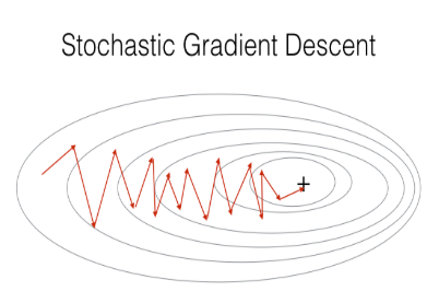
2）Stochastic Gradient Descent，它在每次求梯度的时候只用上一个数据，无疑，这种方式对噪声敏感，且梯度的方向往往偏离较大。

X = data_input

Y = labels

parameters = initialize_parameters(layers_dims)

for i in range(0, num_iterations):

    for j in range(0, m):

        # Forward propagation

        a, caches = forward_propagation(X[:,j], parameters)

        # Compute cost

        cost = compute_cost(a, Y[:,j])

        # Backward propagation

        grads = backward_propagation(a, caches, parameters)

        # Update parameters.

        parameters = update_parameters(parameters, grads)

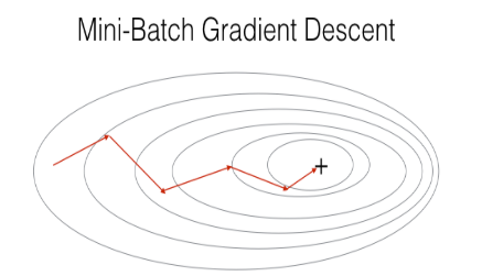
3）Mini-Batch Gradient Descent，就是是在计算梯度时，仅仅利用数据集中的一部分，而不是全部。这样在忽略了梯度准确性的代价下，提升了梯度下降收敛的速度。mini-batch适合用在数据集规模庞大的时。由此可知，min-batch gradient descent 在 batch gradient descent 和 stochastic gradient descent 这两个极端之前采取了折衷的方式，这样既考虑到了梯度的精确性，又考虑到了训练速度，或许这就是中庸之道。

2.执行min-batch gradient descent之前，需要对数据集进行两步操作

1）Shuffle，即打乱数据集的顺序，以此保证数据集随机地分配到mini-batches中。

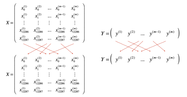
2）Partition，即把数据集分成多个大小相等batches，由于数据集大小可能不被batch size整除，所以最后一个batch的大小可能小于batch size。

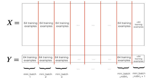
代码如下：

# GRADED FUNCTION: random_mini_batches

def random_mini_batches(X, Y, mini_batch_size = 64, seed = 0):

    """

    Creates a list of random minibatches from (X, Y)

    Arguments:

    X -- input data, of shape (input size, number of examples)

    Y -- true "label" vector (1 for blue dot / 0 for red dot), of shape (1, number of examples)

    mini_batch_size -- size of the mini-batches, integer

    Returns:

    mini_batches -- list of synchronous (mini_batch_X, mini_batch_Y)

    """

    np.random.seed(seed)            # To make your "random" minibatches the same as ours

    m = X.shape[1]                  # number of training examples

    mini_batches = []

    # Step 1: Shuffle (X, Y)

    permutation = list(np.random.permutation(m))

    shuffled_X = X[:, permutation]

    shuffled_Y = Y[:, permutation].reshape((1,m))

    # Step 2: Partition (shuffled_X, shuffled_Y). Minus the end case.

    num_complete_minibatches = math.floor(m/mini_batch_size) # number of mini batches of size mini_batch_size in your partitionning

    for k in range(0, num_complete_minibatches):

        ### START CODE HERE ### (approx. 2 lines)

        mini_batch_X = shuffled_X[:,k*mini_batch_size:(k+1)*mini_batch_size]

        mini_batch_Y = shuffled_Y[:,k*mini_batch_size : (k+1)*mini_batch_size]

        ### END CODE HERE ###

        mini_batch = (mini_batch_X, mini_batch_Y)

        mini_batches.append(mini_batch)

    # Handling the end case (last mini-batch < mini_batch_size)

    if m % mini_batch_size != 0:

        ### START CODE HERE ### (approx. 2 lines)

        mini_batch_X = shuffled_X[:,num_complete_minibatches*mini_batch_size:]

        mini_batch_Y = shuffled_Y[:,num_complete_minibatches*mini_batch_size:]

        ### END CODE HERE ###

        mini_batch = (mini_batch_X, mini_batch_Y)

        mini_batches.append(mini_batch)

    return mini_batches

二.Momentum

1.由于min-batch GD在一次迭代求梯度时，只是用了部分数据集，这就不可避免地导致了梯度出现了偏差（因为掌握的信息不足以作出最明智的选择），由此使得在梯度下降的过程中出现了轻微震荡，如下图在纵向出现了震荡，而momentum可以很好地解决这个问题。

2.momentum的核心思想就是指数加权平均，最通俗的解释就是：在求当前的梯度时，把前面一部分的梯度也考虑进来，然后通过权值计算求和，最终确定当前的梯度。与普通gradient descent的每次求梯度都是相互独立的不同，momentum对于当前的梯度加入了“经验”的元素，且如果某一轴出现了震荡，那么“正反经验”相互抵消，慢慢地梯度方向也趋于平滑，最终达到消除震荡的效果。

3.那如何用数学表达式去实现momentum呢？如下：

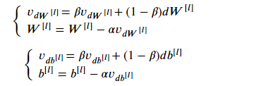
这里引入了v变量，即velocity速度的缩写。那么这个变量与速度又有什么关联？这里或许可以用物理的思想去考虑：dW就是加速度、vdW就是速度。由第一条式子可知，vdW的当前值受到原始速度vdW和加速度dW的加权影响，这样vdW就综合了两者的因素。然后在看第二个式子：W减去学习率乘以vdW，而vdW就是“过往经验”和“当前情况”的综合考虑。

代码如下（v可初始化为0，超级参数 β 一般设置为0.9）：

# GRADED FUNCTION: update_parameters_with_momentum

def update_parameters_with_momentum(parameters, grads, v, beta, learning_rate):

    """

    Update parameters using Momentum

    Arguments:

    parameters -- python dictionary containing your parameters:

                    parameters['W' + str(l)] = Wl

                    parameters['b' + str(l)] = bl

    grads -- python dictionary containing your gradients for each parameters:

                    grads['dW' + str(l)] = dWl

                    grads['db' + str(l)] = dbl

    v -- python dictionary containing the current velocity:

                    v['dW' + str(l)] = ...

                    v['db' + str(l)] = ...

    beta -- the momentum hyperparameter, scalar

    learning_rate -- the learning rate, scalar

    Returns:

    parameters -- python dictionary containing your updated parameters

    v -- python dictionary containing your updated velocities

    """

    L = len(parameters) // 2 # number of layers in the neural networks

    # Momentum update for each parameter

    for l in range(L):

        ### START CODE HERE ### (approx. 4 lines)

        # compute velocities

        v["dW" + str(l+1)] = beta * v["dW" + str(l+1)] + (1-beta) * grads["dW" + str(l+1)]

        v["db" + str(l+1)] = beta * v["db" + str(l+1)] + (1-beta) * grads["db" + str(l+1)]

        # update parameters

        parameters["W" + str(l+1)] = parameters["W" + str(l+1)] - learning_rate * v["dW" + str(l+1)]

        parameters["b" + str(l+1)] = parameters["b" + str(l+1)] - learning_rate * v["db" + str(l+1)]

        ### END CODE HERE ###

    return parameters, v

3.指数加权平均的偏差修正：指数加权平均有一个问题，细看表达式：，一般地v初始化为0，β初始化为0.9，所以v一开始是非常小的，要到后面才进入轨道。如下图，绿色曲线是理想中的曲线，但实际的曲线为紫色曲线：

为了解决这个问题，需要引入修正：即在计算完之后，v还有除以一个系数（1-β^t），即 v = v / (1-β^t)，其中t是当前迭代次数。一开始时β^t小于1但接近于1，于是(1-β^t)就是一个比较小的数，v除以它之后，就能够增大数值，随着迭代次数t的增加β^t接近于0，v / (1-β^t) 就约等于v / 1，即在v进入轨道之后，修正就不再其作用，从而起到对前面的值有修正的作用。

四.RMSprop

1.momentum解决震荡的问题，但是所谓精益求精，我们想在距离长的一方向轴上加速，在距离短的一方向轴上减速。如下图，w轴距离长二b轴距离短：

2.根据上图，可以注意到：距离长的一轴，其斜率小（平缓）；距离短的一轴，其斜率大（陡峭）。因此可以：当斜率大时，将斜率除以一个大的数；当斜率小时，反之。RMSprop的具体做法如下：

五.Adam

Adam则是moment和RMSprop的综合（且加入了修正），即能避免震荡，又能自动调速。其数学表达是：

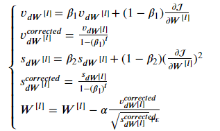
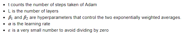
对于上面的几个超级参数，一般如下设置：

初始化v、s（一般初始化为0）：

# GRADED FUNCTION: initialize_adam

def initialize_adam(parameters) :

    """

    Initializes v and s as two python dictionaries with:

                - keys: "dW1", "db1", ..., "dWL", "dbL"

                - values: numpy arrays of zeros of the same shape as the corresponding gradients/parameters.

    Arguments:

    parameters -- python dictionary containing your parameters.

                    parameters["W" + str(l)] = Wl

                    parameters["b" + str(l)] = bl

    Returns:

    v -- python dictionary that will contain the exponentially weighted average of the gradient.

                    v["dW" + str(l)] = ...

                    v["db" + str(l)] = ...

    s -- python dictionary that will contain the exponentially weighted average of the squared gradient.

                    s["dW" + str(l)] = ...

                    s["db" + str(l)] = ...

    """

    L = len(parameters) // 2 # number of layers in the neural networks

    v = {}

    s = {}

    # Initialize v, s. Input: "parameters". Outputs: "v, s".

    for l in range(L):

    ### START CODE HERE ### (approx. 4 lines)

        v["dW" + str(l+1)] = np.zeros( parameters["W" + str(l+1)].shape)

        v["db" + str(l+1)] = np.zeros( parameters["b" + str(l+1)].shape)

        s["dW" + str(l+1)] = np.zeros( parameters["W" + str(l+1)].shape)

        s["db" + str(l+1)] = np.zeros( parameters["b" + str(l+1)].shape)

    ### END CODE HERE ###

    return v, s

Adam更新参数：

# GRADED FUNCTION: update_parameters_with_adam

def update_parameters_with_adam(parameters, grads, v, s, t, learning_rate = 0.01,

                                beta1 = 0.9, beta2 = 0.999,  epsilon = 1e-8):

    """

    Update parameters using Adam

    Arguments:

    parameters -- python dictionary containing your parameters:

                    parameters['W' + str(l)] = Wl

                    parameters['b' + str(l)] = bl

    grads -- python dictionary containing your gradients for each parameters:

                    grads['dW' + str(l)] = dWl

                    grads['db' + str(l)] = dbl

    v -- Adam variable, moving average of the first gradient, python dictionary

    s -- Adam variable, moving average of the squared gradient, python dictionary

    learning_rate -- the learning rate, scalar.

    beta1 -- Exponential decay hyperparameter for the first moment estimates

    beta2 -- Exponential decay hyperparameter for the second moment estimates

    epsilon -- hyperparameter preventing division by zero in Adam updates

    Returns:

    parameters -- python dictionary containing your updated parameters

    v -- Adam variable, moving average of the first gradient, python dictionary

    s -- Adam variable, moving average of the squared gradient, python dictionary

    """

    L = len(parameters) // 2                 # number of layers in the neural networks

    v_corrected = {}                         # Initializing first moment estimate, python dictionary

    s_corrected = {}                         # Initializing second moment estimate, python dictionary

    # Perform Adam update on all parameters

    for l in range(L):

        # Moving average of the gradients. Inputs: "v, grads, beta1". Output: "v".

        ### START CODE HERE ### (approx. 2 lines)

        v["dW" + str(l+1)] = beta1 * v["dW" + str(l+1)] + (1-beta1) * grads["dW" + str(l+1)]

        v["db" + str(l+1)] = beta1 * v["db" + str(l+1)] + (1-beta1) * grads["db" + str(l+1)]

        ### END CODE HERE ###

        # Compute bias-corrected first moment estimate. Inputs: "v, beta1, t". Output: "v_corrected".

        ### START CODE HERE ### (approx. 2 lines)

        v_corrected["dW" + str(l+1)] = v["dW" + str(l+1)]/(1-beta1**t)

        v_corrected["db" + str(l+1)] = v["db" + str(l+1)]/(1-beta1**t)

        ### END CODE HERE ###

        # Moving average of the squared gradients. Inputs: "s, grads, beta2". Output: "s".

        ### START CODE HERE ### (approx. 2 lines)

        s["dW" + str(l+1)] = beta2 * s["dW" + str(l+1)] + (1-beta2) * grads["dW" + str(l+1)]**2

        s["db" + str(l+1)] = beta2 * s["db" + str(l+1)] + (1-beta2) * grads["db" + str(l+1)]**2

        ### END CODE HERE ###

        # Compute bias-corrected second raw moment estimate. Inputs: "s, beta2, t". Output: "s_corrected".

        ### START CODE HERE ### (approx. 2 lines)

        s_corrected["dW" + str(l+1)] = s["dW" + str(l+1)]/(1-beta2**t)

        s_corrected["db" + str(l+1)] = s["db" + str(l+1)]/(1-beta2**t)

        ### END CODE HERE ###

        # Update parameters. Inputs: "parameters, learning_rate, v_corrected, s_corrected, epsilon". Output: "parameters".

        ### START CODE HERE ### (approx. 2 lines)

        parameters["W" + str(l+1)] = parameters["W" + str(l+1)] - learning_rate * v_corrected["dW" + str(l+1)]/(s_corrected["dW" + str(l+1)]+epsilon)**0.5

        parameters["b" + str(l+1)] = parameters["b" + str(l+1)] - learning_rate * v_corrected["db" + str(l+1)]/(s_corrected["db" + str(l+1)]+epsilon)**0.5

        ### END CODE HERE ###

    return parameters, v, s

六.优化算法性能比较

接下来分别用mini-batch gradient descent 、 momentum 、 Adam 来对模型进行训练，并比较三者的性能。

模型如下（需要接收一个参数更新的方式）：

# GRADED FUNCTION: update_parameters_with_adam

def update_parameters_with_adam(parameters, grads, v, s, t, learning_rate = 0.01,

                                beta1 = 0.9, beta2 = 0.999,  epsilon = 1e-8):

    """

    Update parameters using Adam

    Arguments:

    parameters -- python dictionary containing your parameters:

                    parameters['W' + str(l)] = Wl

                    parameters['b' + str(l)] = bl

    grads -- python dictionary containing your gradients for each parameters:

                    grads['dW' + str(l)] = dWl

                    grads['db' + str(l)] = dbl

    v -- Adam variable, moving average of the first gradient, python dictionary

    s -- Adam variable, moving average of the squared gradient, python dictionary

    learning_rate -- the learning rate, scalar.

    beta1 -- Exponential decay hyperparameter for the first moment estimates

    beta2 -- Exponential decay hyperparameter for the second moment estimates

    epsilon -- hyperparameter preventing division by zero in Adam updates

    Returns:

    parameters -- python dictionary containing your updated parameters

    v -- Adam variable, moving average of the first gradient, python dictionary

    s -- Adam variable, moving average of the squared gradient, python dictionary

    """

    L = len(parameters) // 2                 # number of layers in the neural networks

    v_corrected = {}                         # Initializing first moment estimate, python dictionary

    s_corrected = {}                         # Initializing second moment estimate, python dictionary

    # Perform Adam update on all parameters

    for l in range(L):

        # Moving average of the gradients. Inputs: "v, grads, beta1". Output: "v".

        ### START CODE HERE ### (approx. 2 lines)

        v["dW" + str(l+1)] = beta1 * v["dW" + str(l+1)] + (1-beta1) * grads["dW" + str(l+1)]

        v["db" + str(l+1)] = beta1 * v["db" + str(l+1)] + (1-beta1) * grads["db" + str(l+1)]

        ### END CODE HERE ###

        # Compute bias-corrected first moment estimate. Inputs: "v, beta1, t". Output: "v_corrected".

        ### START CODE HERE ### (approx. 2 lines)

        v_corrected["dW" + str(l+1)] = v["dW" + str(l+1)]/(1-beta1**t)

        v_corrected["db" + str(l+1)] = v["db" + str(l+1)]/(1-beta1**t)

        ### END CODE HERE ###

        # Moving average of the squared gradients. Inputs: "s, grads, beta2". Output: "s".

        ### START CODE HERE ### (approx. 2 lines)

        s["dW" + str(l+1)] = beta2 * s["dW" + str(l+1)] + (1-beta2) * grads["dW" + str(l+1)]**2

        s["db" + str(l+1)] = beta2 * s["db" + str(l+1)] + (1-beta2) * grads["db" + str(l+1)]**2

        ### END CODE HERE ###

        # Compute bias-corrected second raw moment estimate. Inputs: "s, beta2, t". Output: "s_corrected".

        ### START CODE HERE ### (approx. 2 lines)

        s_corrected["dW" + str(l+1)] = s["dW" + str(l+1)]/(1-beta2**t)

        s_corrected["db" + str(l+1)] = s["db" + str(l+1)]/(1-beta2**t)

        ### END CODE HERE ###

        # Update parameters. Inputs: "parameters, learning_rate, v_corrected, s_corrected, epsilon". Output: "parameters".

        ### START CODE HERE ### (approx. 2 lines)

        parameters["W" + str(l+1)] = parameters["W" + str(l+1)] - learning_rate * v_corrected["dW" + str(l+1)]/(s_corrected["dW" + str(l+1)]+epsilon)**0.5

        parameters["b" + str(l+1)] = parameters["b" + str(l+1)] - learning_rate * v_corrected["db" + str(l+1)]/(s_corrected["db" + str(l+1)]+epsilon)**0.5

        ### END CODE HERE ###

    return parameters, v, s

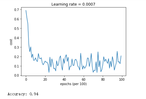
1）mini-batch gradient descent

可见其代价函数抖动得比较厉害，可能这是“mini-batch”这种选取部分数据的方式所无法避免的吧。而且准确率也不高。

2）momentum

momentum居然跟mini-batch gradient descent 的效果无异，在进行理论解释时明明是那么的美好，为什么会这样？

3）Adam

Adam不仅收敛速度快，而且震荡也较之不明显，更重要的是准确率高，性能明显优于mini-batch gradient descent 、 momentum。由此可见，在梯度下降的优化算法方面，Adam做得十分出色！

七.学习率衰减

1.在使用min-batch gradient descent的时候，由于没有使用到全部数据（或者说batch里面存在噪声），梯度下降时方向很可能不是指向局部最优点，而是有些偏差，就像一个醉汉一样颠颠簸簸地往前走，如下图：

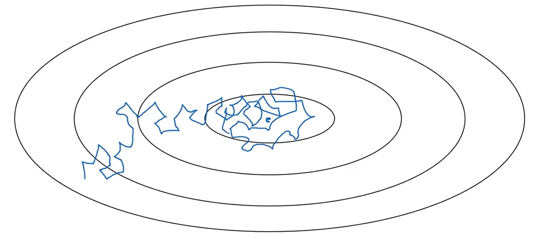
2.在靠近局部走优点的过程中，应该逐渐降低学习率，即以更细的步伐行走，才能更加精确地靠近局部最优点。其过程如下图的绿色曲线：

吴恩达深度学习笔记（五） —— 优化算法：Mini-Batch GD、Momentum、RMSprop、Adam、学习率衰减的更多相关文章

吴恩达深度学习笔记（十二）—— Batch Normalization
主要内容: 一.Normalizing activations in a network 二.Fitting Batch Norm in a neural network 三.Why does ...
【Deeplearning.ai 】吴恩达深度学习笔记及课后作业目录
吴恩达深度学习课程的课堂笔记以及课后作业代码下载:https://github.com/douzujun/Deep-Learning-Coursera 吴恩达推荐笔记:https://mp.weix ...
吴恩达深度学习笔记（八） —— ResNets残差网络
(很好的博客:残差网络ResNet笔记) 主要内容: 一.深层神经网络的优点和缺陷二.残差网络的引入三.残差网络的可行性四.identity block 和 convolutional bloc ...
吴恩达深度学习笔记（deeplearning.ai）之卷积神经网络（二）
经典网络 LeNet-5 AlexNet VGG Ng介绍了上述三个在计算机视觉中的经典网络.网络深度逐渐增加,训练的参数数量也骤增.AlexNet大约6000万参数,VGG大约上亿参数. 从中我们可 ...
吴恩达深度学习笔记（deeplearning.ai）之卷积神经网络（CNN）（上）
作者:szx_spark 1. Padding 在卷积操作中,过滤器(又称核)的大小通常为奇数,如3x3,5x5.这样的好处有两点: 在特征图(二维卷积)中就会存在一个中心像素点.有一个中心像素点会十 ...
吴恩达深度学习笔记（deeplearning.ai）之循环神经网络（RNN）（三）
1. 导读本节内容介绍普通RNN的弊端,从而引入各种变体RNN,主要讲述GRU与LSTM的工作原理. 事先声明,本人采用ng在课堂上所使用的符号系统,与某些学术文献上的命名有所不同,不过核心思想都是 ...
吴恩达深度学习笔记（deeplearning.ai）之卷积神经网络（一）
Padding 在卷积操作中,过滤器(又称核)的大小通常为奇数,如3x3,5x5.这样的好处有两点: 在特征图(二维卷积)中就会存在一个中心像素点.有一个中心像素点会十分方便,便于指出过滤器的位置. ...
吴恩达深度学习笔记（九） —— FaceNet
主要内容: 一.FaceNet人脸识别简介二.使用神经网络对人脸进行编码三.代价函数triple loss 四.人脸库五.人脸认证与人脸识别一.FaceNet简介 1.FaceNet是一个深层 ...
吴恩达深度学习笔记（七） —— Batch Normalization
主要内容: 一.Batch Norm简介二.归一化网络的激活函数三.Batch Norm拟合进神经网络四.测试时的Batch Norm 一.Batch Norm简介 1.在机器学习中,我们一般会 ...

随机推荐

android自定义View_0——Create a custom view class
一:创建一个自定义view的原则: 1.符合android的标准 2.能在layout的xml中定义控件属性 3.实现些新功能 4.要兼容android的大多数版本二:定义一个view的子类 1.可 ...
控制器post参数接收
一.post对象 1.后台c# public class TestController : ApiController { [HttpPost] public string SaveData1(Tb_ ...
Python 对Twitter tweet的元素 (Word, Screen Name, Hash Tag)的频率分析
CODE: #!/usr/bin/python # -*- coding: utf-8 -*- ''' Created on 2014-7-2 @author: guaguastd @name: tw ...
std::condition_variable(3)复习
#include <iostream> // std::cout #include <thread> // std::thread #include <mutex> ...
restful demo 演示; jquery min1.1;
[说明]上午建立了一个restful风格的一个测试,运行通过:下午试了试postman,想看看http请求的具体过程,但是chrome浏览器的network面板也可以查看,并且很方便,就索性用它了一 ...
【转】在服务器上排除问题的头五分钟&常用命令
转自:https://blog.csdn.net/l821133235/article/details/80103106(在服务器上排除问题的头五分钟) 遇到服务器故障,问题出现的原因很少可以一下就想 ...
[转]C#静态方法与非静态方法的比较
http://wenku.baidu.com/view/4e1704084a7302768e9939e0.html C#的类中可以包含两种方法:C#静态方法与非静态方法.那么他们的定义有什么不同呢?他 ...
浅谈Spring框架注解的用法分析
原文出处: locality 1.@Component是Spring定义的一个通用注解,可以注解任何bean. 2.@Scope定义bean的作用域,其默认作用域是”singleton”,除此之外还有 ...
巨蟒django之权限6: 权限控制表设计&&登录权限
1.权限控制表设计内容 . 什么是权限? . 为什么要有权限? 不同用户拥有不同的功能 . 在web开发中,什么是权限? url 代表权限 . 开发一个权限的组件,为什么要开发组件? . 表结构的 ...
2014-08-28——移动端web开发，基本Meta标签
1.<meta name="viewport" content="width=device-width, initial-scale=1, maximum-scal ...

吴恩达深度学习笔记（五） —— 优化算法：Mini-Batch GD、Momentum、RMSprop、Adam、学习率衰减

吴恩达深度学习笔记（五） —— 优化算法：Mini-Batch GD、Momentum、RMSprop、Adam、学习率衰减的更多相关文章

随机推荐

热门专题