利用python绘制分析路易斯安那州巴吞鲁日市的人口密度格局

前言

数据来源于王法辉教授的GIS和数量方法，以后有空，我会利用python来实现里面的案例，这里向王法辉教授致敬。

绘制普查人口密度格局

使用属性查询提取区边界

import numpy as np
import pandas as pd
import geopandas as gpd
import matplotlib.pyplot as plt
import arcpy
from arcpy import env
plt.style.use('ggplot')#使用ggplot样式
%matplotlib inline#输出在线图片

plt.rcParams['font.family'] = ['sans-serif']
plt.rcParams['font.sans-serif'] = ['SimHei']# 替换sans-serif字体为黑体
plt.rcParams['axes.unicode_minus'] = False   # 解决坐标轴负数的负号显示问题

regions = gpd.GeoDataFrame.from_file('../Census.gdb',layer='County')
regions

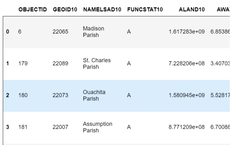
BRTrt = regions[regions.NAMELSAD10=='East Baton Rouge Parish']

投影

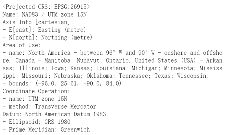
BRTrt = BRTrt.to_crs('EPSG:26915')
BRTrt.crs

BRTrt.to_file('BRTrt.shp')

裁剪数据

Tract = gpd.GeoDataFrame.from_file('../Census.gdb',layer='Tract')
Tract = Tract.to_crs('EPSG:26915')

TractUtm = gpd.GeoDataFrame.from_file('TractUtm.shp')
BRTrtUtm = gpd.GeoDataFrame.from_file('BRTrt.shp')

# Set workspace
env.workspace = r"MyProject"

# Set local variables
in_features = "TractUtm.shp"
clip_features = "BRTrt.shp"
out_feature_class = "BRTrtUtm.shp"
xy_tolerance = ""

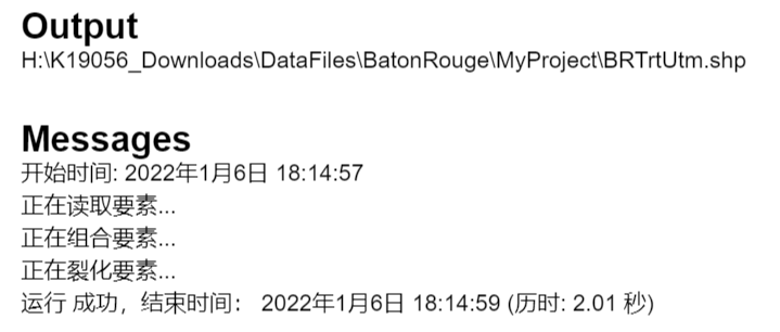
# Execute Clip
arcpy.Clip_analysis(in_features, clip_features, out_feature_class, xy_tolerance)

计算面积和人口密度

BRTrtUtm = gpd.GeoDataFrame.from_file('BRTrtUtm.shp')
BRTrtUtm['area'] = BRTrtUtm.area/1000000

## 计算人口密度
BRTrtUtm['PopuDen'] = BRTrtUtm['DP0010001']/BRTrtUtm['area']
BRTrtUtm.to_file('BRTrtUtm.shp')

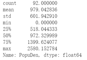
描述统计

BRTrtUtm['PopuDen'].describe()

人口密度图

fig = plt.figure(figsize=(12,12)) #设置画布大小
ax = plt.gca()
ax.set_title("巴吞鲁日市2010年人口密度模式",fontsize=24,loc='center')
BRTrtUtm.plot(ax=ax,column='PopuDen',linewidth=0.5,cmap='Reds'
              ,edgecolor='k',legend=True,)
# plt.savefig('巴吞鲁日市2010年人口密度模式.jpg',dpi=300)

plt.show()

分析同心环区的人口密度格式

生成同心环

## 两种方法生成多重缓冲区的阈值
dis = list(np.arange(2000,26001,2000))
dis
dis = list(range(2000,26001,2000))
dis

## 真的特别神奇distances只有这样写列表才可以运行

# Set local variables
inFeatures = "BRCenter"
outFeatureClass = "rings.shp"
distances = [2000, 4000, 6000, 8000, 10000,
             12000, 14000, 16000, 18000,
             20000, 22000, 24000, 26000]
bufferUnit = "meters"

# Execute MultipleRingBuffer
arcpy.MultipleRingBuffer_analysis(inFeatures, outFeatureClass, distances, bufferUnit, "", "ALL")

相交

try:
    # Set the workspace (to avoid having to type in the full path to the data every time)
    arcpy.env.workspace = "MyProject"    

    # Process: Find all stream crossings (points)
    inFeatures = ["rings", "BRTrtUtm"]
    intersectOutput = "TrtRings.shp"
    arcpy.Intersect_analysis(inFeatures, intersectOutput,)

except Exception as err:
    print(err.args[0])

TrtRings = gpd.GeoDataFrame.from_file('TrtRings.shp')
TrtRings['area'] = TrtRings.area/1000000

TrtRings['EstPopu'] = TrtRings['PopuDen'] * TrtRings['POLY_AREA']

融合

arcpy.env.workspace = "C:/data/Portland.gdb/Taxlots"

# Set local variables
inFeatures = "TrtRings"
outFeatureClass = "DissRings.shp"
dissolveFields = ["distance"]
statistics_fields = [["POLY_AREA","SUM"], ["PopuDen","SUM"]]

# Execute Dissolve using LANDUSE and TAXCODE as Dissolve Fields

arcpy.Dissolve_management(inFeatures, outFeatureClass, dissolveFields, statistics_fields,)

DissRings = gpd.GeoDataFrame.from_file('DissRings.shp')
DissRings

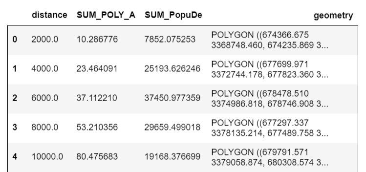
DissRings['PopuDen'] = DissRings['SUM_PopuDe'] / DissRings['SUM_POLY_A']
DissRings.set_index('distance',inplace=True)

DissRings['PopuDen'].plot(kind='bar',x='distance',
                          xlabel='',figsize=(8,6))
plt.savefig('同心环人口密度图.jpg',dpi=300)
plt.show()

要素转点

# Set environment settings
env.workspace = "BR.gdb"

#  Set local variables
inFeatures = "BRBlkUtm"
outFeatureClass = "BRBlkPt.shp"

# Use FeatureToPoint function to find a point inside each park
arcpy.FeatureToPoint_management(inFeatures, outFeatureClass, "INSIDE")

标识

env.workspace = "MyProject"

# Set local parameters
inFeatures = "BRBlkPt"
idFeatures = "DissRings"
outFeatures = "BRBlkPt_Identity.shp"

# Process: Use the Identity function
arcpy.Identity_analysis(inFeatures, idFeatures, outFeatures)

数据筛选

BRBlkPt_Identity = gpd.GeoDataFrame.from_file('BRBlkPt_Identity.shp')
BRBlkPt_Identity.shape

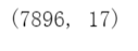
BRBlkPt_Identity.tail()

## 选取数据
BRBlkPt_Identity = BRBlkPt_Identity[~(BRBlkPt_Identity['distance']==0.0)]

数据分组

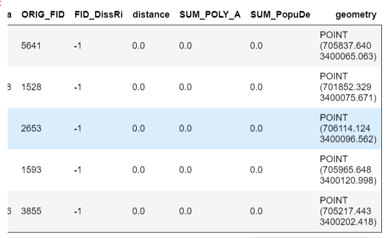
rigs_data = pd.DataFrame(BRBlkPt_Identity.groupby(by=['distance'])['POP10'].sum(),columns=['POP10'])
rigs_data.reset_index(inplace=True)
rigs_data

数据连接

EstPopu = BRBlkPt_Identity[['distance','SUM_POLY_A','SUM_PopuDe']]
PopuDen = pd.merge(rigs_data,EstPopu,how='inner',left_on='distance',right_on='distance')

## 删除重复值，按理来说，应该没有重复值了，可以试试外连接
PopuDen.drop_duplicates(inplace = True)

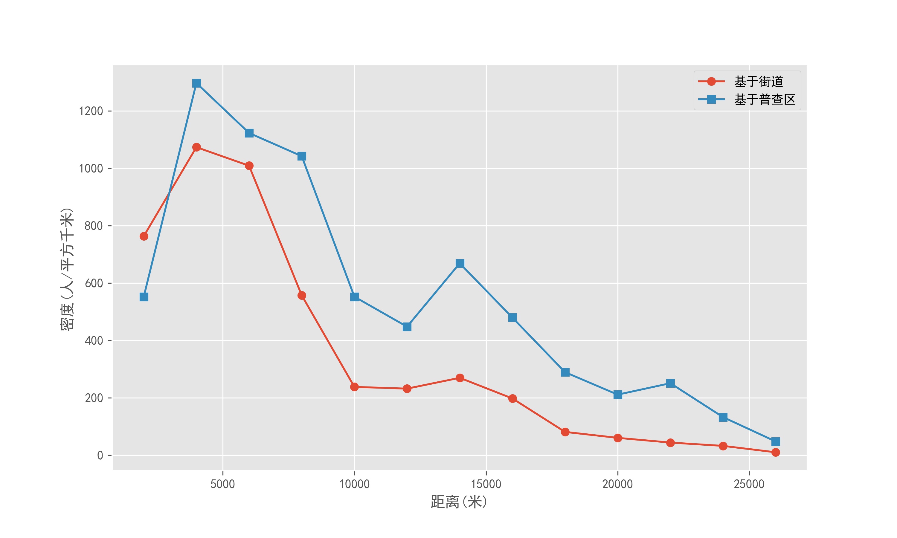
分析和比较环形区人口和密度估值

PopuDen.set_index('distance',inplace=True)
PopuDen['EstPopu'] = PopuDen['SUM_PopuDe'] / PopuDen['SUM_POLY_A']
PopuDen['PopuDen1'] = PopuDen['POP10'] / PopuDen['SUM_POLY_A']

PopuDen['EstPopu'].plot(figsize=(10,6),marker='o',xlabel='距离(米)',ylabel='密度(人/平方千米)')
PopuDen['PopuDen1'].plot(marker='s',xlabel='距离(米)',ylabel='密度(人/平方千米)')

plt.legend(['基于街道','基于普查区'])
plt.savefig('基于普查区和街区数据的人口密度模式对比.jpg',dpi=300)
plt.show()

总结

2022年的第一次写笔记，写的不是很好，而且发现许多问题，比如就是geopandas里面的area和arcpy里面的area不一样，可能是算法不一样，面积要使用投影坐标系，我相信这个应该没有人不知道了吧，要对ArcGIS Pro里面的arcpy大赞。最近感谢也比较多，比如疫情，已经有点常态化，很影响我们的生活了。心怀感恩，希望我们都有美好的未来。春燕归，巢于林木。接下来一段时间，我要忙我的毕业论文，可能会比较忙，需要数据的可以联系我。