《DSP using MATLAB》Problem 7.12

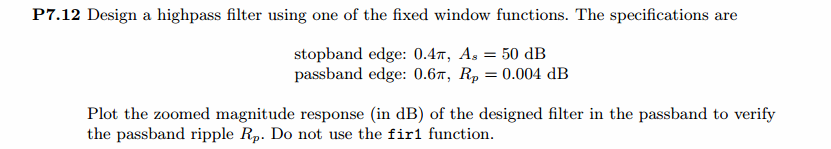
阻带衰减50dB，我们选Hamming窗

代码：

%% ++++++++++++++++++++++++++++++++++++++++++++++++++++++++++++++++++++++++++++++++
%%            Output Info about this m-file
fprintf('\n***********************************************************\n');
fprintf('        <DSP using MATLAB> Problem 7.12 \n\n');

banner();
%% ++++++++++++++++++++++++++++++++++++++++++++++++++++++++++++++++++++++++++++++++

% highpass
ws1 = 0.4*pi; wp1 = 0.6*pi; As = 50; Rp = 0.004;
tr_width = (wp1-ws1);
M = ceil(6.6*pi/tr_width) + 1;                 % Hamming Window
fprintf('\nFilter Length: M = %d.\n', M);

n = [0:1:M-1]; wc1 = (ws1+wp1)/2; 

%wc = (ws + wp)/2,                    % ideal LPF cutoff frequency

hd = ideal_lp(pi, M) - ideal_lp(wc1, M);
w_hamm = (hamming(M))';  h = hd .* w_hamm;
[db, mag, pha, grd, w] = freqz_m(h, [1]);  delta_w = 2*pi/1000;
[Hr,ww,P,L] = ampl_res(h);

Rp = -(min(db(wp1/delta_w+1 :1: 0.9*pi/delta_w)));              % Actual Passband Ripple
fprintf('\nActual Passband Ripple is %.4f dB.\n', Rp);

As = -round(max(db(1 :1: ws1/delta_w+1 )));          % Min Stopband attenuation
fprintf('\nMin Stopband attenuation is %.4f dB.\n', As);

[delta1, delta2] = db2delta(Rp, As)

% Plot

figure('NumberTitle', 'off', 'Name', 'Problem 7.12 ideal_lp Method')
set(gcf,'Color','white'); 

subplot(2,2,1); stem(n, hd); axis([0 M-1 -0.4 0.3]); grid on;
xlabel('n'); ylabel('hd(n)'); title('Ideal Impulse Response');

subplot(2,2,2); stem(n, w_hamm); axis([0 M-1 0 1.1]); grid on;
xlabel('n'); ylabel('w(n)'); title('Hamming Window');

subplot(2,2,3); stem(n, h); axis([0 M-1 -0.4 0.3]); grid on;
xlabel('n'); ylabel('h(n)'); title('Actual Impulse Response');

subplot(2,2,4); plot(w/pi, db); axis([0 1 -100 10]); grid on;
set(gca,'YTickMode','manual','YTick',[-90,-52,0]);
set(gca,'YTickLabelMode','manual','YTickLabel',['90';'52';' 0']);
set(gca,'XTickMode','manual','XTick',[0,0.4,0.6,1]);
xlabel('frequency in \pi units'); ylabel('Decibels'); title('Magnitude Response in dB');

figure('NumberTitle', 'off', 'Name', 'Problem 7.12 h(n) ideal_lp Method')
set(gcf,'Color','white'); 

subplot(2,2,1); plot(w/pi, db); grid on; axis([0 2 -100 10]);
xlabel('frequency in \pi units'); ylabel('Decibels'); title('Magnitude Response in dB');
set(gca,'YTickMode','manual','YTick',[-90,-52,0])
set(gca,'YTickLabelMode','manual','YTickLabel',['90';'52';' 0']);
set(gca,'XTickMode','manual','XTick',[0,0.4,0.6,1,1.4,1.6,2]);

subplot(2,2,3); plot(w/pi, mag); grid on; %axis([0 2 -100 10]);
xlabel('frequency in \pi units'); ylabel('Absolute'); title('Magnitude Response in absolute');
set(gca,'XTickMode','manual','XTick',[0,0.4,0.6,1,1.4,1.6,2]);
set(gca,'YTickMode','manual','YTick',[0.0,0.5,1.0])

subplot(2,2,2); plot(w/pi, pha); grid on; %axis([0 1 -100 10]);
xlabel('frequency in \pi units'); ylabel('Rad'); title('Phase Response in Radians');
subplot(2,2,4); plot(w/pi, grd*pi/180);  grid on; %axis([0 1 -100 10]);
xlabel('frequency in \pi units'); ylabel('Rad'); title('Group Delay');

figure('NumberTitle', 'off', 'Name', 'Problem 7.12 h(n)')
set(gcf,'Color','white'); 

plot(ww/pi, Hr); grid on; %axis([0 1 -100 10]);
xlabel('frequency in \pi units'); ylabel('Hr'); title('Amplitude Response');
set(gca,'YTickMode','manual','YTick',[-delta2,0,delta2,1 - delta1,1, 1 + delta1])
%set(gca,'YTickLabelMode','manual','YTickLabel',['90';'45';' 0']);
%set(gca,'XTickMode','manual','XTick',[0,0.4,0.6,1,1.4,1.6,2]);

h_check = fir1(M, wc1/pi, 'high');
[db, mag, pha, grd, w] = freqz_m(h_check, [1]);
[Hr,ww,P,L] = ampl_res(h_check);

figure('NumberTitle', 'off', 'Name', 'Problem 7.12 fir1 Method')
set(gcf,'Color','white'); 

subplot(2,2,1); stem(n, hd); axis([0 M-1 -0.4 0.3]); grid on;
xlabel('n'); ylabel('hd(n)'); title('Ideal Impulse Response');

subplot(2,2,2); stem(n, w_hamm); axis([0 M-1 0 1.1]); grid on;
xlabel('n'); ylabel('w(n)'); title('Hanning Window');

subplot(2,2,3); stem([0:M], h_check); axis([0 M -0.4 0.5]); grid on;
xlabel('n'); ylabel('h\_check(n)'); title('Actual Impulse Response');

subplot(2,2,4); plot(w/pi, db); axis([0 1 -100 10]); grid on;
set(gca,'YTickMode','manual','YTick',[-90,-52,0])
set(gca,'YTickLabelMode','manual','YTickLabel',['90';'52';' 0']);
set(gca,'XTickMode','manual','XTick',[0,0.4,0.6,1]);
xlabel('frequency in \pi units'); ylabel('Decibels'); title('Magnitude Response in dB');

figure('NumberTitle', 'off', 'Name', 'Problem 7.12 h(n) fir1 Method')
set(gcf,'Color','white'); 

subplot(2,2,1); plot(w/pi, db); grid on; axis([0 2 -100 10]);
xlabel('frequency in \pi units'); ylabel('Decibels'); title('Magnitude Response in dB');
set(gca,'YTickMode','manual','YTick',[-90,-52,0])
set(gca,'YTickLabelMode','manual','YTickLabel',['90';'52';' 0']);
set(gca,'XTickMode','manual','XTick',[0,0.4,0.6,1,1.4,1.6,2]);

subplot(2,2,3); plot(w/pi, mag); grid on; %axis([0 1 -100 10]);
xlabel('frequency in \pi units'); ylabel('Absolute'); title('Magnitude Response in absolute');
set(gca,'XTickMode','manual','XTick',[0,0.4,0.6,1,1.4,1.6,2]);
set(gca,'YTickMode','manual','YTick',[0.0,0.5,1.0])

subplot(2,2,2); plot(w/pi, pha); grid on; %axis([0 1 -100 10]);
xlabel('frequency in \pi units'); ylabel('Rad'); title('Phase Response in Radians');
subplot(2,2,4); plot(w/pi, grd*pi/180);  grid on; %axis([0 1 -100 10]);
xlabel('frequency in \pi units'); ylabel('Rad'); title('Group Delay');

　　运行结果：

Hamming窗长度为M=34，实际最小阻带衰减为52dB，满足设计要求。

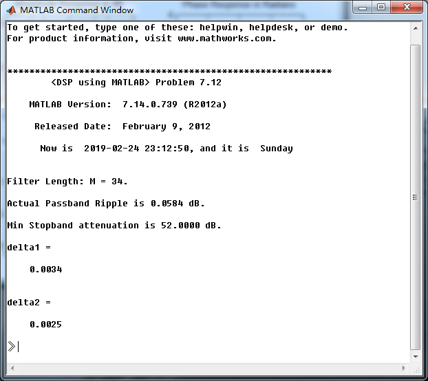
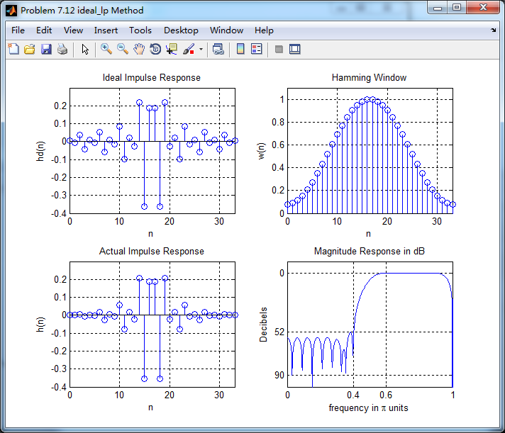
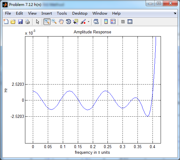
振幅响应的高通部分

低阻部分

下面是用fir1函数（默认Hamming窗）来求得脉冲响应，再计算其幅度响应（dB和Absolute单位）、相位响应和群延迟响应，

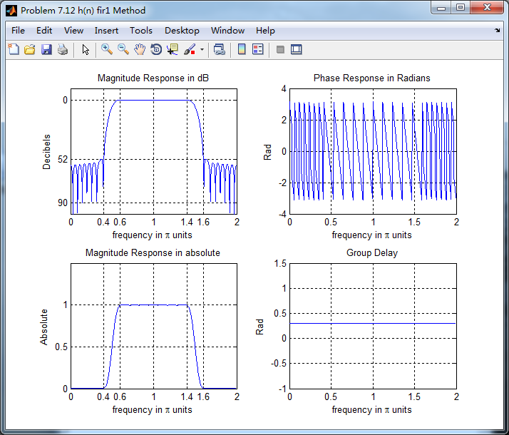
可以看出，两种方法得到的幅度响应和相位响应在接近π的较高频率部分，还是有差别的。