吴裕雄--天生自然 R语言开发学习：聚类分析

#-------------------------------------------------------#
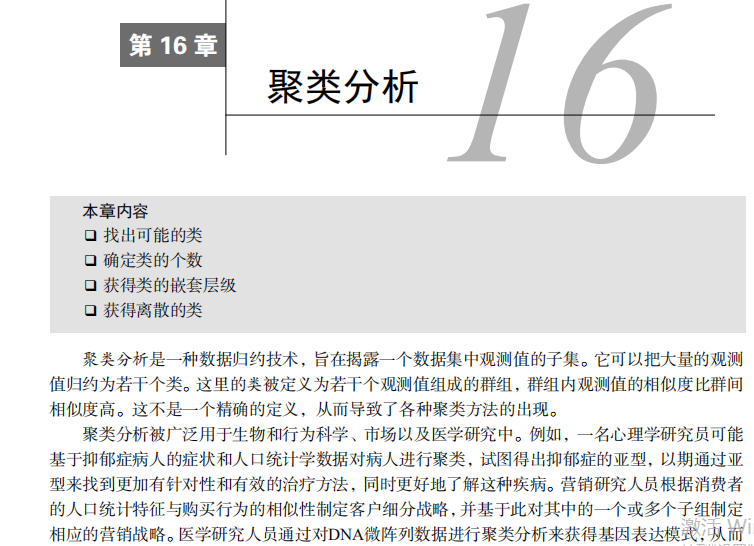
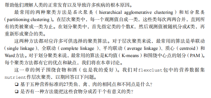
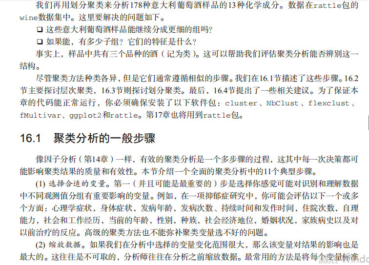
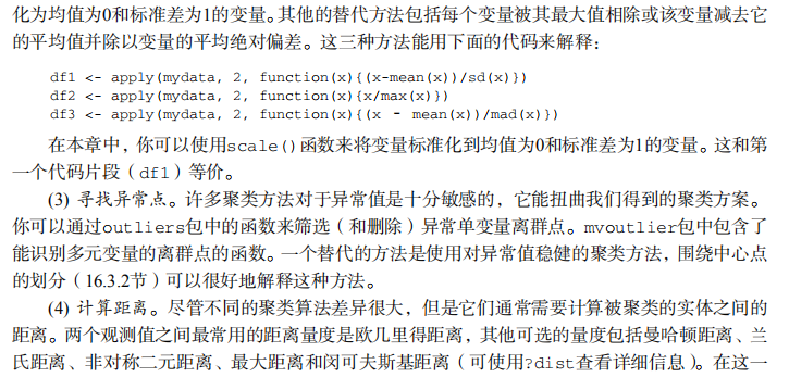
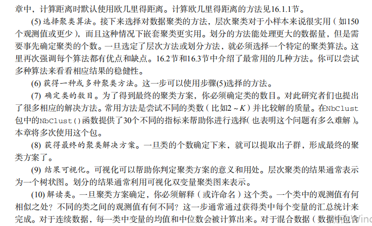
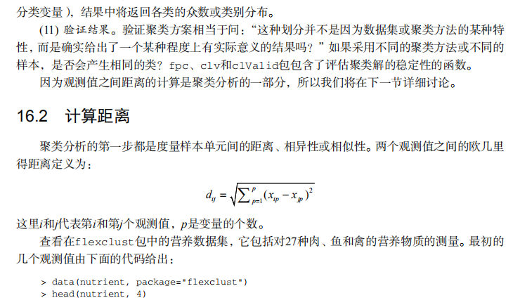
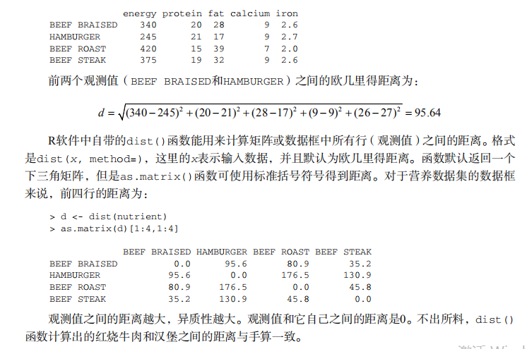
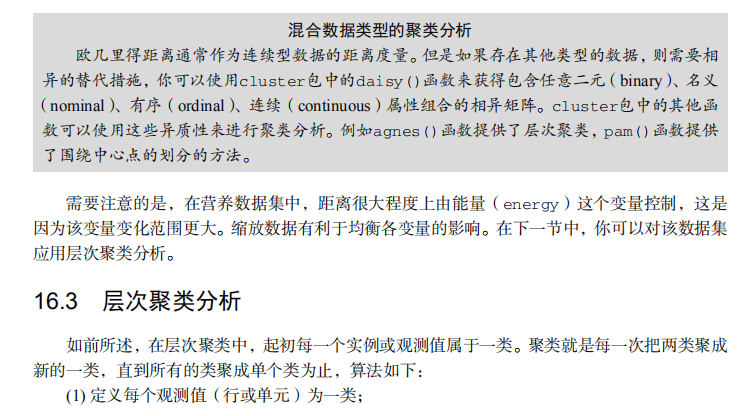
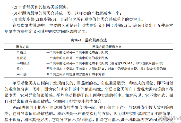
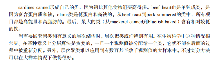
# R in Action (2nd ed): Chapter 16                      #
# Cluster analysis                                      #
# requires packaged NbClust, flexclust, rattle          #
# install.packages(c("NbClust", "flexclust", "rattle")) #
#-------------------------------------------------------#

par(ask=TRUE)
opar <- par(no.readonly=FALSE)

# Calculating Distances
data(nutrient, package="flexclust")
head(nutrient, 2)
d <- dist(nutrient)
as.matrix(d)[1:4,1:4]

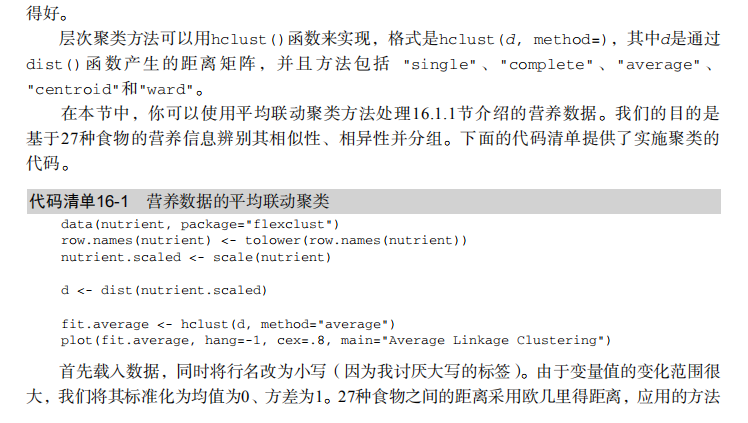
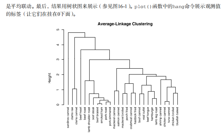
# Listing 16.1 - Average linkage clustering of nutrient data
data(nutrient, package="flexclust")
row.names(nutrient) <- tolower(row.names(nutrient))
nutrient.scaled <- scale(nutrient)
d <- dist(nutrient.scaled)
fit.average <- hclust(d, method="average")
plot(fit.average, hang=-1, cex=.8, main="Average Linkage Clustering")

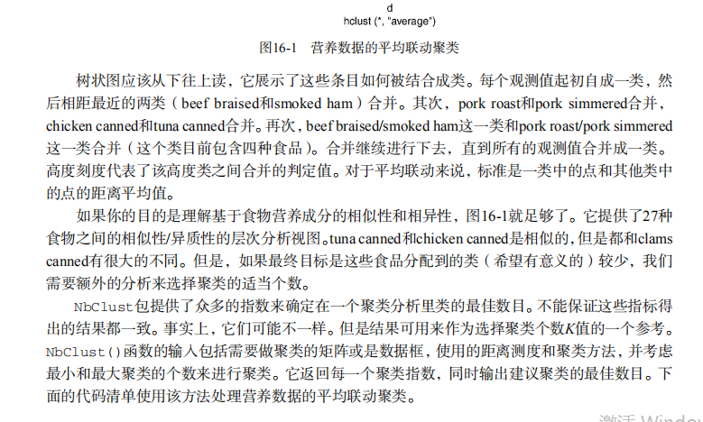
# Listing 16.2 - Selecting the number of clusters
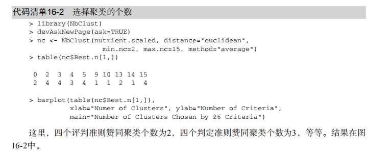
library(NbClust)
nc <- NbClust(nutrient.scaled, distance="euclidean",
              min.nc=2, max.nc=15, method="average")
par(opar)
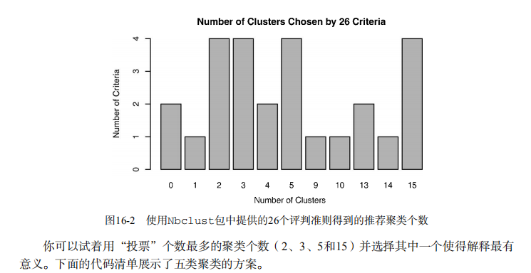
table(nc$Best.n[1,])
barplot(table(nc$Best.n[1,]),
        xlab="Numer of Clusters", ylab="Number of Criteria",
        main="Number of Clusters Chosen by 26 Criteria") 

# Listing 16.3 - Obtaining the final cluster solution
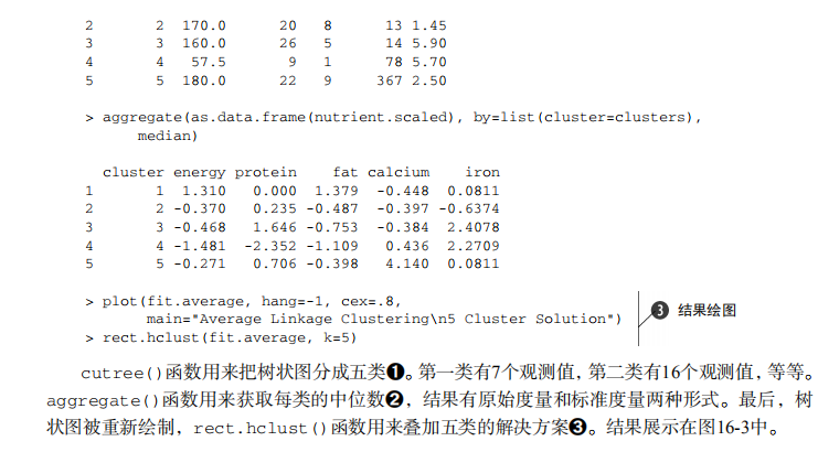
clusters <- cutree(fit.average, k=5)
table(clusters)
aggregate(nutrient, by=list(cluster=clusters), median)
aggregate(as.data.frame(nutrient.scaled), by=list(cluster=clusters),
          median)
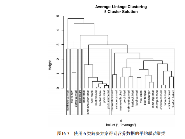
plot(fit.average, hang=-1, cex=.8,
     main="Average Linkage Clustering\n5 Cluster Solution")
rect.hclust(fit.average, k=5)

# Plot function for within groups sum of squares by number of clusters
wssplot <- function(data, nc=15, seed=1234){
  wss <- (nrow(data)-1)*sum(apply(data,2,var))
  for (i in 2:nc){
    set.seed(seed)
    wss[i] <- sum(kmeans(data, centers=i)$withinss)}
  plot(1:nc, wss, type="b", xlab="Number of Clusters",
       ylab="Within groups sum of squares")}

# Listing 16.4 - K-means clustering of wine data
data(wine, package="rattle")
head(wine)
df <- scale(wine[-1])
wssplot(df)
library(NbClust)
set.seed(1234)
nc <- NbClust(df, min.nc=2, max.nc=15, method="kmeans")
par(opar)
table(nc$Best.n[1,])
barplot(table(nc$Best.n[1,]),
        xlab="Numer of Clusters", ylab="Number of Criteria",
        main="Number of Clusters Chosen by 26 Criteria")
set.seed(1234)
fit.km <- kmeans(df, 3, nstart=25)
fit.km$size
fit.km$centers
aggregate(wine[-1], by=list(cluster=fit.km$cluster), mean)

# evaluate clustering
ct.km <- table(wine$Type, fit.km$cluster)
ct.km
library(flexclust)
randIndex(ct.km)

# Listing 16.5 - Partitioning around mediods for the wine data
library(cluster)
set.seed(1234)
fit.pam <- pam(wine[-1], k=3, stand=TRUE)
fit.pam$medoids
clusplot(fit.pam, main="Bivariate Cluster Plot")

# evaluate clustering
ct.pam <- table(wine$Type, fit.pam$clustering)
ct.pam
randIndex(ct.pam)

## Avoiding non-existent clusters
library(fMultivar)
set.seed(1234)
df <- rnorm2d(1000, rho=.5)
df <- as.data.frame(df)
plot(df, main="Bivariate Normal Distribution with rho=0.5")

wssplot(df)
library(NbClust)
nc <- NbClust(df, min.nc=2, max.nc=15, method="kmeans")
par(opar)
barplot(table(nc$Best.n[1,]),
        xlab="Numer of Clusters", ylab="Number of Criteria",
        main  ="Number of Clusters Chosen by 26 Criteria")

library(ggplot2)
library(cluster)
fit <- pam(df, k=2)
df$clustering <- factor(fit$clustering)
ggplot(data=df, aes(x=V1, y=V2, color=clustering, shape=clustering)) +
  geom_point() + ggtitle("Clustering of Bivariate Normal Data")

plot(nc$All.index[,4], type="o", ylab="CCC",
     xlab="Number of clusters", col="blue")