《DSP using MATLAB》示例Example 8.23

代码：

%% ------------------------------------------------------------------------
%%            Output Info about this m-file
fprintf('\n***********************************************************\n');
fprintf('        <DSP using MATLAB> Exameple 8.23 \n\n');

time_stamp = datestr(now, 31);
[wkd1, wkd2] = weekday(today, 'long');
fprintf('      Now is %20s, and it is %8s  \n\n', time_stamp, wkd2);
%% ------------------------------------------------------------------------

% Digital Filter Specifications:
wp = 0.2*pi;                 % digital passband freq in rad
ws = 0.3*pi;                 % digital stopband freq in rad
Rp = 1;                      % passband ripple in dB
As = 15;                     % stopband attenuation in dB

% Analog prototype specifications: Inverse Mapping for frequencies
T = 1;                           % set T = 1
OmegaP = (2/T)*tan(wp/2);        % Prewarp(Cutoff) prototype passband freq
OmegaS = (2/T)*tan(ws/2);        % Prewarp(cutoff) prototype stopband freq

% Analog Prototype Order Calculations:
ep = sqrt(10^(Rp/10)-1);           % Passband Ripple Factor
A = 10^(As/20);                    % Stopband Attenuation Factor
OmegaC = OmegaP;                   % Analog Chebyshev-2 prototype cutoff freq
OmegaR = OmegaS/OmegaP;            % Analog prototype Transition ratio
g = sqrt(A*A-1)/ep;                % Analog prototype Intermediate cal

N  = ceil(log10(g+sqrt(g*g-1))/log10(OmegaR+sqrt(OmegaR*OmegaR-1)));
fprintf('\n\n ********** Chebyshev-2 Filter Order = %3.0f  \n', N)

% Digital Chebyshev-2 Filter Design:
wn = ws/pi;                        % Digital Chebyshev-2 cutoff freq in pi units

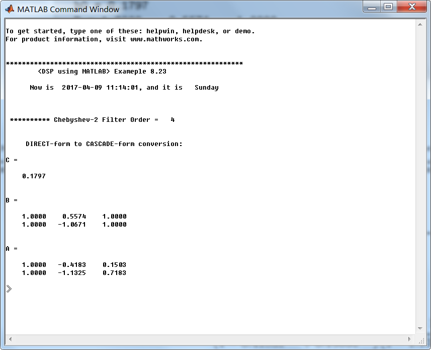
[b, a] = cheby2(N, As, wn); [C, B, A] = dir2cas(b, a)

% Calculation of Frequency Response:
[db, mag, pha, grd, ww] = freqz_m(b, a);

%% -----------------------------------------------------------------
%%                             Plot
%% -----------------------------------------------------------------  

figure('NumberTitle', 'off', 'Name', 'Exameple 8.23')
set(gcf,'Color','white');
M = 1;                          % Omega max

subplot(2,2,1); plot(ww/pi, mag); axis([0, M, 0, 1.2]); grid on;
xlabel(' frequency in \pi units'); ylabel('|H|'); title('Magnitude Response');
set(gca, 'XTickMode', 'manual', 'XTick', [0, 0.2, 0.3, M]);
set(gca, 'YTickMode', 'manual', 'YTick', [0, 0.1778, 0.8913, 1]);

subplot(2,2,2); plot(ww/pi, pha/pi); axis([0, M, -1.1, 1.1]); grid on;
xlabel('frequency in \pi nuits'); ylabel('radians in \pi units'); title('Phase Response');
set(gca, 'XTickMode', 'manual', 'XTick', [0, 0.2, 0.3, M]);
set(gca, 'YTickMode', 'manual', 'YTick', [-1:1:1]);

subplot(2,2,3); plot(ww/pi, db); axis([0, M, -30, 10]); grid on;
xlabel('frequency in \pi units'); ylabel('Decibels'); title('Magnitude in dB ');
set(gca, 'XTickMode', 'manual', 'XTick', [0, 0.2, 0.3, M]);
set(gca, 'YTickMode', 'manual', 'YTick', [-30, -15, -1, 0]);

subplot(2,2,4); plot(ww/pi, grd); axis([0, M, 0, 15]); grid on;
xlabel('frequency in \pi units'); ylabel('Samples'); title('Group Delay');
set(gca, 'XTickMode', 'manual', 'XTick', [0, 0.2, 0.3, M]);
set(gca, 'YTickMode', 'manual', 'YTick', [0:5:15]);

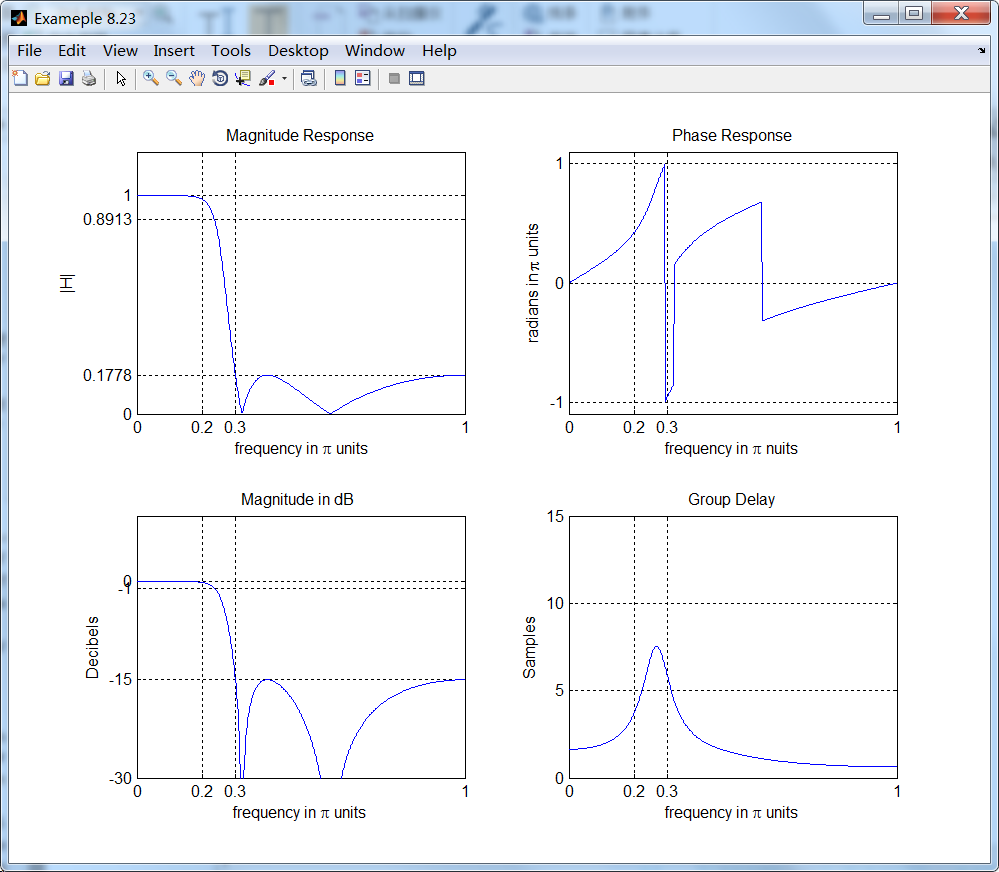
　　运行结果：