cluster KMeans need preprocessing scale????

Out:

n_digits: 10,    n_samples 1797,         n_features 64
__________________________________________________________________________________
init            time    inertia homo    compl   v-meas  ARI     AMI     silhouette
k-means++       0.30s   69432   0.602   0.650   0.625   0.465   0.598   0.146
random          0.23s   69694   0.669   0.710   0.689   0.553   0.666   0.147
PCA-based       0.04s   70804   0.671   0.698   0.684   0.561   0.668   0.118
__________________________________________________________________________________

 from:http://scikit-learn.org/stable/auto_examples/cluster/plot_kmeans_digits.html#sphx-glr-auto-examples-cluster-plot-kmeans-digits-py

print(__doc__)

from time import time
import numpy as np
import matplotlib.pyplot as plt

from sklearn import metrics
from sklearn.cluster import KMeans
from sklearn.datasets import load_digits
from sklearn.decomposition import PCA
from sklearn.preprocessing import scale

np.random.seed(42)

digits = load_digits()
data = scale(digits.data)

n_samples, n_features = data.shape
n_digits = len(np.unique(digits.target))
labels = digits.target

sample_size = 300

print("n_digits: %d, \t n_samples %d, \t n_features %d"
      % (n_digits, n_samples, n_features))

print(82 * '_')
print('init\t\ttime\tinertia\thomo\tcompl\tv-meas\tARI\tAMI\tsilhouette')

def bench_k_means(estimator, name, data):
    t0 = time()
    estimator.fit(data)
    print('%-9s\t%.2fs\t%i\t%.3f\t%.3f\t%.3f\t%.3f\t%.3f\t%.3f'
          % (name, (time() - t0), estimator.inertia_,
             metrics.homogeneity_score(labels, estimator.labels_),
             metrics.completeness_score(labels, estimator.labels_),
             metrics.v_measure_score(labels, estimator.labels_),
             metrics.adjusted_rand_score(labels, estimator.labels_),
             metrics.adjusted_mutual_info_score(labels,  estimator.labels_),
             metrics.silhouette_score(data, estimator.labels_,
                                      metric='euclidean',
                                      sample_size=sample_size)))

bench_k_means(KMeans(init='k-means++', n_clusters=n_digits, n_init=10),
              name="k-means++", data=data)

bench_k_means(KMeans(init='random', n_clusters=n_digits, n_init=10),
              name="random", data=data)

# in this case the seeding of the centers is deterministic, hence we run the
# kmeans algorithm only once with n_init=1
pca = PCA(n_components=n_digits).fit(data)
bench_k_means(KMeans(init=pca.components_, n_clusters=n_digits, n_init=1),
              name="PCA-based",
              data=data)
print(82 * '_')

# #############################################################################
# Visualize the results on PCA-reduced data

reduced_data = PCA(n_components=2).fit_transform(data)
kmeans = KMeans(init='k-means++', n_clusters=n_digits, n_init=10)
kmeans.fit(reduced_data)

# Step size of the mesh. Decrease to increase the quality of the VQ.
h = .02     # point in the mesh [x_min, x_max]x[y_min, y_max].

# Plot the decision boundary. For that, we will assign a color to each
x_min, x_max = reduced_data[:, 0].min() - 1, reduced_data[:, 0].max() + 1
y_min, y_max = reduced_data[:, 1].min() - 1, reduced_data[:, 1].max() + 1
xx, yy = np.meshgrid(np.arange(x_min, x_max, h), np.arange(y_min, y_max, h))

# Obtain labels for each point in mesh. Use last trained model.
Z = kmeans.predict(np.c_[xx.ravel(), yy.ravel()])

# Put the result into a color plot
Z = Z.reshape(xx.shape)
plt.figure(1)
plt.clf()
plt.imshow(Z, interpolation='nearest',
           extent=(xx.min(), xx.max(), yy.min(), yy.max()),
           cmap=plt.cm.Paired,
           aspect='auto', origin='lower')

plt.plot(reduced_data[:, 0], reduced_data[:, 1], 'k.', markersize=2)
# Plot the centroids as a white X
centroids = kmeans.cluster_centers_
plt.scatter(centroids[:, 0], centroids[:, 1],
            marker='x', s=169, linewidths=3,
            color='w', zorder=10)
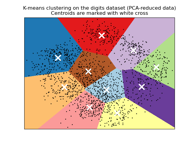
plt.title('K-means clustering on the digits dataset (PCA-reduced data)\n'
          'Centroids are marked with white cross')
plt.xlim(x_min, x_max)
plt.ylim(y_min, y_max)
plt.xticks(())
plt.yticks(())
plt.show()

It depends on your data.

If you have attributes with a well-defined meaning. Say, latitude and longitude, then you should not scale your data, because this will cause distortion. (K-means might be a bad choice, too - you need something that can handle lat/lon naturally)

If you have mixed numerical data, where each attribute is something entirely different (say, shoe size and weight), has different units attached (lb, tons, m, kg ...) then these values aren't really comparable anyway; z-standardizing them is a best-practise to give equal weight to them.

If you have binary values, discrete attributes or categorial attributes, stay away from k-means. K-means needs to compute means, and the mean value is not meaningful on this kind of data.

from:https://stats.stackexchange.com/questions/89809/is-it-important-to-scale-data-before-clustering

Importance of Feature Scaling

Feature scaling though standardization (or Z-score normalization) can be an important preprocessing step for many machine learning algorithms. Standardization involves rescaling the features such that they have the properties of a standard normal distribution with a mean of zero and a standard deviation of one.

While many algorithms (such as SVM, K-nearest neighbors, and logistic regression) require features to be normalized, intuitively we can think of Principle Component Analysis (PCA) as being a prime example of when normalization is important. In PCA we are interested in the components that maximize the variance. If one component (e.g. human height) varies less than another (e.g. weight) because of their respective scales (meters vs. kilos), PCA might determine that the direction of maximal variance more closely corresponds with the ‘weight’ axis, if those features are not scaled. As a change in height of one meter can be considered much more important than the change in weight of one kilogram, this is clearly incorrect.

To illustrate this, PCA is performed comparing the use of data with StandardScaler applied, to unscaled data. The results are visualized and a clear difference noted. The 1st principal component in the unscaled set can be seen. It can be seen that feature #13 dominates the direction, being a whole two orders of magnitude above the other features. This is contrasted when observing the principal component for the scaled version of the data. In the scaled version, the orders of magnitude are roughly the same across all the features.

The dataset used is the Wine Dataset available at UCI. This dataset has continuous features that are heterogeneous in scale due to differing properties that they measure (i.e alcohol content, and malic acid).

The transformed data is then used to train a naive Bayes classifier, and a clear difference in prediction accuracies is observed wherein the dataset which is scaled before PCA vastly outperforms the unscaled version.

from:http://scikit-learn.org/stable/auto_examples/preprocessing/plot_scaling_importance.html