矩池云 | 使用LightGBM来预测分子属性

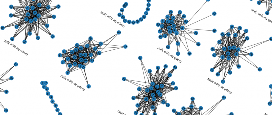
今天给大家介绍提升方法(Boosting), 提升算法是一种可以用来减小监督式学习中偏差的机器学习算法。

面对的问题是迈可·肯斯（Michael Kearns）提出的：一组“弱学习者”的集合能否生成一个“强学习者”？

弱学习者一般是指一个分类器，它的结果只比随机分类好一点点。强学习者指分类器的结果非常接近真值。

大多数提升算法包括由迭代使用弱学习分类器组成，并将其结果加入一个最终的成强学习分类器。加入的过程中，通常根据它们的分类准确率给予不同的权重。加和弱学习者之后，数据通常会被重新加权，来强化对之前分类错误数据点的分类。

提升算法有种三个臭皮匠顶个诸葛亮的意思。在这里将使用微软的LightGBM这个提升算法，来预测分子的一个属性，叫做耦合常数。

导入需要的库

import os

import time

import datetime

import json

import gc

from numba import jit

import pandas as pd

import numpy as np

import matplotlib.pyplot as plt

%matplotlib inline

from tqdm import tqdm_notebook

from sklearn.preprocessing import StandardScaler

from sklearn.svm import NuSVR, SVR

from sklearn.metrics import mean_absolute_error

pd.options.display.precision = 15

import lightgbm as lgb

import xgboost as xgb

from catboost import CatBoostRegressor

from sklearn.preprocessing import LabelEncoder

from sklearn.model_selection import StratifiedKFold, KFold, RepeatedKFold

from sklearn import metrics

from sklearn import linear_model

import seaborn as sns

import warnings

warnings.filterwarnings("ignore")

from IPython.display import HTML

import altair as alt

from altair.vega import v5

from IPython.display import HTML

import networkx as nx

import matplotlib.pyplot as plt

%matplotlib inline

alt.renderers.enable('notebook')

读取数据

读取需要使用的csv文件，

train = pd.read_csv('train.csv')

test = pd.read_csv('test.csv')

structures = pd.read_csv('structures.csv')

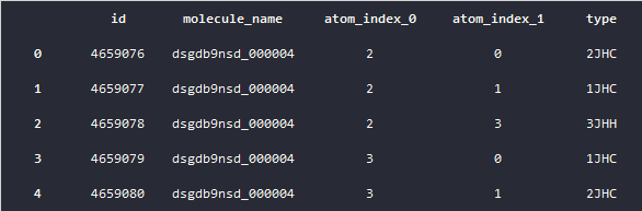
csv文件中包含了以下这些数据，首先看下训练集的数据，从pandas显示的数据来看，训练集的csv包含了，分子名，原子index，化学键类型和训练集给出的耦合常数。

train.head()

在测试集数据中，除了耦合常数的数据其他的数据跟训练集的数据是一致的。

test.head()

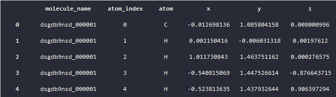
再来看下structures的数据，也就是原子的数据，其中包含了，原子的索引，这个原子在哪个分子中，和它的空间坐标位置，这些数据后续将会用来做特征挖掘。

structures.head()

可数据化的数据

数据可视化一直是机器学习的重点，一个好的数据可视化，可以帮助我们理解数据的分布、形态以及特性。

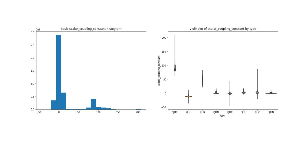
首先来看下耦合常数在已有的数据集中分布，这里展示了耦合常数的直方图，以及每个化学键类型下的耦合常数的数据大小的分布情况。

fig, ax = plt.subplots(figsize = (18, 6))

plt.subplot(1, 2, 1);

plt.hist(train['scalar_coupling_constant'], bins=20);

plt.title('Basic scalar_coupling_constant histogram');

plt.subplot(1, 2, 2);

sns.violinplot(x='type', y='scalar_coupling_constant', data=train);

plt.title('Violinplot of scalar_coupling_constant by type');

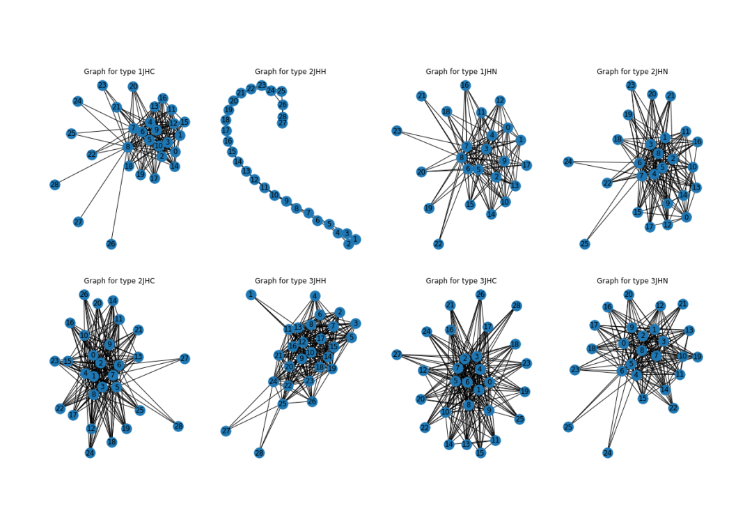
再来看下已有的数据，根据不同的化学键类型的原子连接形态。

从图表中可以发现，不同给的化学键类型，有着不同的形态，其中2JHH这个化学键的形态最为特别。

fig, ax = plt.subplots(figsize = (20, 12))

for i, t in enumerate(train['type'].unique()):

    train_type = train.loc[train['type'] == t]

    G = nx.from_pandas_edgelist(train_type, 'atom_index_0', 'atom_index_1', ['scalar_coupling_constant'])

    plt.subplot(2, 4, i + 1);

    nx.draw(G, with_labels=True);

    plt.title(f'Graph for type {t}')

特征工程

提升算法，一般的数据形式都是基于表单的数据。比如说这次的案例中分子与原子的数据。

对于这类数据，最重要的一个工作就是特征工程，如何从现有的特征中挖掘出其他有价值的特征将是这类算法的最大的难点。下面我们做一些简单的特征工程，来展示下特征工程的过程，

首先，将结构表跟训练数据表和测试数据表进行合并。



def map_atom_info(df, atom_idx):

    df = pd.merge(df, structures, how = 'left',

                  left_on  = ['molecule_name', f'atom_index_{atom_idx}'],

                  right_on = ['molecule_name',  'atom_index'])

    df = df.drop('atom_index', axis=1)

    df = df.rename(columns={'atom': f'atom_{atom_idx}',

                            'x': f'x_{atom_idx}',

                            'y': f'y_{atom_idx}',

                            'z': f'z_{atom_idx}'})

    return df

train = map_atom_info(train, 0)

train = map_atom_info(train, 1)

test = map_atom_info(test, 0)

test = map_atom_info(test, 1)

观察合并以后的数据，发现原子的类型以及空间位置都合并到了训练集数据和测试集数据相应的行中。

train.head()

test.head()

计算距离特征

分别计算训练集和测试集数据集中，每一行中两个原子间的距离特征，其中包括，

原子距离；
原子x上的距离；
原子y上的距离；
原子z上的距离；

并且把这些距离合并到训练集和测试集数据集上，

train_p_0 = train[['x_0', 'y_0', 'z_0']].values

train_p_1 = train[['x_1', 'y_1', 'z_1']].values

test_p_0 = test[['x_0', 'y_0', 'z_0']].values

test_p_1 = test[['x_1', 'y_1', 'z_1']].values

train['dist'] = np.linalg.norm(train_p_0 - train_p_1, axis=1)

test['dist'] = np.linalg.norm(test_p_0 - test_p_1, axis=1)

train['dist_x'] = (train['x_0'] - train['x_1']) ** 2

test['dist_x'] = (test['x_0'] - test['x_1']) ** 2

train['dist_y'] = (train['y_0'] - train['y_1']) ** 2

test['dist_y'] = (test['y_0'] - test['y_1']) ** 2

train['dist_z'] = (train['z_0'] - train['z_1']) ** 2

test['dist_z'] = (test['z_0'] - test['z_1']) ** 2

计算每种化学键的距离的均值，

train['type_0'] = train['type'].apply(lambda x: x[0])

test['type_0'] = test['type'].apply(lambda x: x[0])

train['type_1'] = train['type'].apply(lambda x: x[1:])

test['type_1'] = test['type'].apply(lambda x: x[1:])

train['type_0'] = train['type'].apply(lambda x: x[0])

test['type_0'] = test['type'].apply(lambda x: x[0])

train['type_1'] = train['type'].apply(lambda x: x[1:])

test['type_1'] = test['type'].apply(lambda x: x[1:])

train['dist_to_type_mean'] = train['dist'] / train.groupby('type')['dist'].transform('mean')

test['dist_to_type_mean'] = test['dist'] / test.groupby('type')['dist'].transform('mean')

train['dist_to_type_0_mean'] = train['dist'] / train.groupby('type_0')['dist'].transform('mean')

test['dist_to_type_0_mean'] = test['dist'] / test.groupby('type_0')['dist'].transform('mean')

train['dist_to_type_1_mean'] = train['dist'] / train.groupby('type_1')['dist'].transform('mean')

test['dist_to_type_1_mean'] = test['dist'] / test.groupby('type_1')['dist'].transform('mean')

将化学键以分子为单位进行分组并计算分子均值，

train[f'molecule_type_dist_mean'] = train.groupby(['molecule_name', 'type'])['dist'].transform('mean')

test[f'molecule_type_dist_mean'] = test.groupby(['molecule_name', 'type'])['dist'].transform('mean')

将原子与化学键类型编码成数值，方便后续训练。

for f in ['atom_0', 'atom_1', 'type_0', 'type_1', 'type']:

    lbl = LabelEncoder()

    lbl.fit(list(train[f].values) + list(test[f].values))

    train[f] = lbl.transform(list(train[f].values))

    test[f] = lbl.transform(list(test[f].values))

准备数据

首先排除一些我们不需要的列数据，

X = train.drop(['id', 'molecule_name', 'scalar_coupling_constant'], axis=1)

y = train['scalar_coupling_constant']

X_test = test.drop(['id', 'molecule_name'], axis=1)

然后将数据分拆成几个fold，每个fold的数据都会打乱。

n_fold = 5

folds = KFold(n_splits=n_fold, shuffle=True, random_state=11)

定义模型

特征工程完成之后，就需要定义我们的模型，这里我们使用LightGBM来训练。

LigthGBM是boosting集合模型中的新进成员，由微软提供，它和XGBoost一样是对GBDT的高效实现，原理上它和GBDT及XGBoost类似，都采用损失函数的负梯度作为当前决策树的残差近似值，去拟合新的决策树。

LightGBM在很多方面会比XGBoost表现的更为优秀，比如：更快的训练效率；低内存使用；更高的准确率；支持并行化学习可处理大规模数据；支持直接使用category特征等。

首先我们需要设置LightGBM的参数

LightGBM的参数很多，在这里对某几个关键的参数做下解释

max_depth：树模型深度；

num_leaves：叶子节点数，数模型复杂度；

min_child_samples：表示一个叶子节点上包含的最少样本数量；

objective：目标函数；

learning_rate：学习率；

max_depth：控制了树的最大深度。该参数可以显式的限制树的深度；

boosting_type：给出了基学习器模型算法；

params = {'num_leaves': 128,

          'min_child_samples': 79,

          'objective': 'regression',

          'max_depth': 13,

          'learning_rate': 0.2,

          "boosting_type": "gbdt",

          "subsample_freq": 1,

          "subsample": 0.9,

          "bagging_seed": 11,

          "metric": 'mae',

          "verbosity": -1,

          'reg_alpha': 0.1,

          'reg_lambda': 0.3,

          'colsample_bytree': 1.0

         }

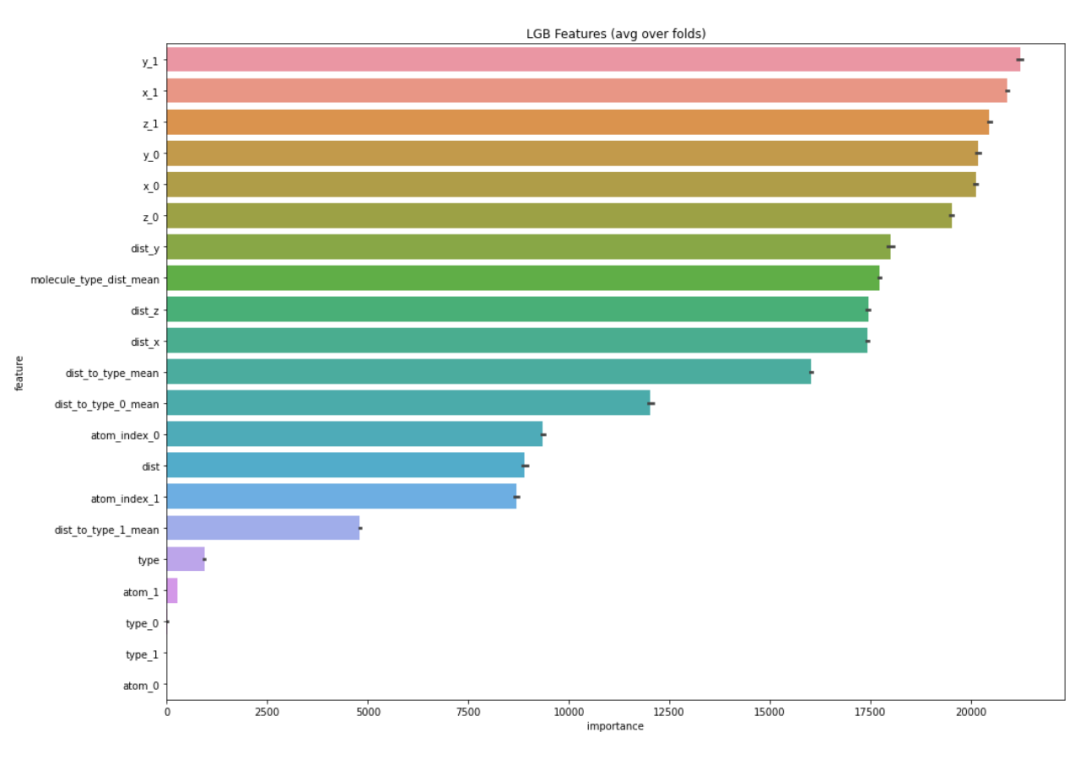
定义训练函数, 在训练函数里记录了每个特征的重要性，并在训练结束后通过图表展示，有助于筛选特征。

def group_mean_log_mae(y_true, y_pred, types, floor=1e-9):

    maes = (y_true-y_pred).abs().groupby(types).mean()

    return np.log(maes.map(lambda x: max(x, floor))).mean()

def train_model_regression(X, X_test, y, params, folds, model_type='lgb', eval_metric='mae', columns=None, plot_feature_importance=False, model=None,

                           verbose=10000, early_stopping_rounds=200, n_estimators=50000):

    columns = X.columns if columns is None else columns

    X_test = X_test[columns]

    # to set up scoring parameters

    metrics_dict = {'mae': {'lgb_metric_name': 'mae',

                        'catboost_metric_name': 'MAE',

                        'sklearn_scoring_function': metrics.mean_absolute_error},

                    'group_mae': {'lgb_metric_name': 'mae',

                        'catboost_metric_name': 'MAE',

                        'scoring_function': group_mean_log_mae},

                    'mse': {'lgb_metric_name': 'mse',

                        'catboost_metric_name': 'MSE',

                        'sklearn_scoring_function': metrics.mean_squared_error}

                    }

    result_dict = {}

    # out-of-fold predictions on train data

    oof = np.zeros(len(X))

    # averaged predictions on train data

    prediction = np.zeros(len(X_test))

    # list of scores on folds

    scores = []

    feature_importance = pd.DataFrame()

    # split and train on folds

    for fold_n, (train_index, valid_index) in enumerate(folds.split(X)):

        print(f'Fold {fold_n + 1} started at {time.ctime()}')

        if type(X) == np.ndarray:

            X_train, X_valid = X[columns][train_index], X[columns][valid_index]

            y_train, y_valid = y[train_index], y[valid_index]

        else:

            X_train, X_valid = X[columns].iloc[train_index], X[columns].iloc[valid_index]

            y_train, y_valid = y.iloc[train_index], y.iloc[valid_index]

        if model_type == 'lgb':

            model = lgb.LGBMRegressor(**params, n_estimators = n_estimators, n_jobs = -1)

            model.fit(X_train, y_train,

                    eval_set=[(X_train, y_train), (X_valid, y_valid)], eval_metric=metrics_dict[eval_metric]['lgb_metric_name'],

                    verbose=verbose, early_stopping_rounds=early_stopping_rounds)

            y_pred_valid = model.predict(X_valid)

            y_pred = model.predict(X_test, num_iteration=model.best_iteration_)

        if model_type == 'xgb':

            train_data = xgb.DMatrix(data=X_train, label=y_train, feature_names=X.columns)

            valid_data = xgb.DMatrix(data=X_valid, label=y_valid, feature_names=X.columns)

            watchlist = [(train_data, 'train'), (valid_data, 'valid_data')]

            model = xgb.train(dtrain=train_data, num_boost_round=20000, evals=watchlist, early_stopping_rounds=200, verbose_eval=verbose, params=params)

            y_pred_valid = model.predict(xgb.DMatrix(X_valid, feature_names=X.columns), ntree_limit=model.best_ntree_limit)

            y_pred = model.predict(xgb.DMatrix(X_test, feature_names=X.columns), ntree_limit=model.best_ntree_limit)

        if model_type == 'sklearn':

            model = model

            model.fit(X_train, y_train)

            y_pred_valid = model.predict(X_valid).reshape(-1,)

            score = metrics_dict[eval_metric]['sklearn_scoring_function'](y_valid, y_pred_valid)

            print(f'Fold {fold_n}. {eval_metric}: {score:.4f}.')

            print('')

            y_pred = model.predict(X_test).reshape(-1,)

        if model_type == 'cat':

            model = CatBoostRegressor(iterations=20000,  eval_metric=metrics_dict[eval_metric]['catboost_metric_name'], **params,

                                      loss_function=metrics_dict[eval_metric]['catboost_metric_name'])

            model.fit(X_train, y_train, eval_set=(X_valid, y_valid), cat_features=[], use_best_model=True, verbose=False)

            y_pred_valid = model.predict(X_valid)

            y_pred = model.predict(X_test)

        oof[valid_index] = y_pred_valid.reshape(-1,)

        if eval_metric != 'group_mae':

            scores.append(metrics_dict[eval_metric]['sklearn_scoring_function'](y_valid, y_pred_valid))

        else:

            scores.append(metrics_dict[eval_metric]['scoring_function'](y_valid, y_pred_valid, X_valid['type']))

        prediction += y_pred    

        if model_type == 'lgb' and plot_feature_importance:

            # feature importance

            fold_importance = pd.DataFrame()

            fold_importance["feature"] = columns

            fold_importance["importance"] = model.feature_importances_

            fold_importance["fold"] = fold_n + 1

            feature_importance = pd.concat([feature_importance, fold_importance], axis=0)

    prediction /= folds.n_splits

    print('CV mean score: {0:.4f}, std: {1:.4f}.'.format(np.mean(scores), np.std(scores)))

    result_dict['oof'] = oof

    result_dict['prediction'] = prediction

    result_dict['scores'] = scores

    if model_type == 'lgb':

        if plot_feature_importance:

            feature_importance["importance"] /= folds.n_splits

            cols = feature_importance[["feature", "importance"]].groupby("feature").mean().sort_values(

                by="importance", ascending=False)[:50].index

            best_features = feature_importance.loc[feature_importance.feature.isin(cols)]

            plt.figure(figsize=(16, 12));

            sns.barplot(x="importance", y="feature", data=best_features.sort_values(by="importance", ascending=False));

            plt.title('LGB Features (avg over folds)');

            result_dict['feature_importance'] = feature_importance

    return result_dict

开始训练

在训练结束的时候，会输出每个特征值的重要程度，柱状图越长，表明这个特征在预测时候所起到的作用越大。

通过重要性的观察，可以帮助我们筛选出较好的特征，剔除一些不太重要的特征。一来特征越少训练速度越快，二来保留重要的特征不会对结果有较大影响。

result_dict_lgb = train_model_regression(X=X, X_test=X_test, y=y, params=params, folds=folds, model_type='lgb', eval_metric='group_mae', plot_feature_importance=True,

                                                      verbose=1000, early_stopping_rounds=200, n_estimators=10000)

预测结果分布

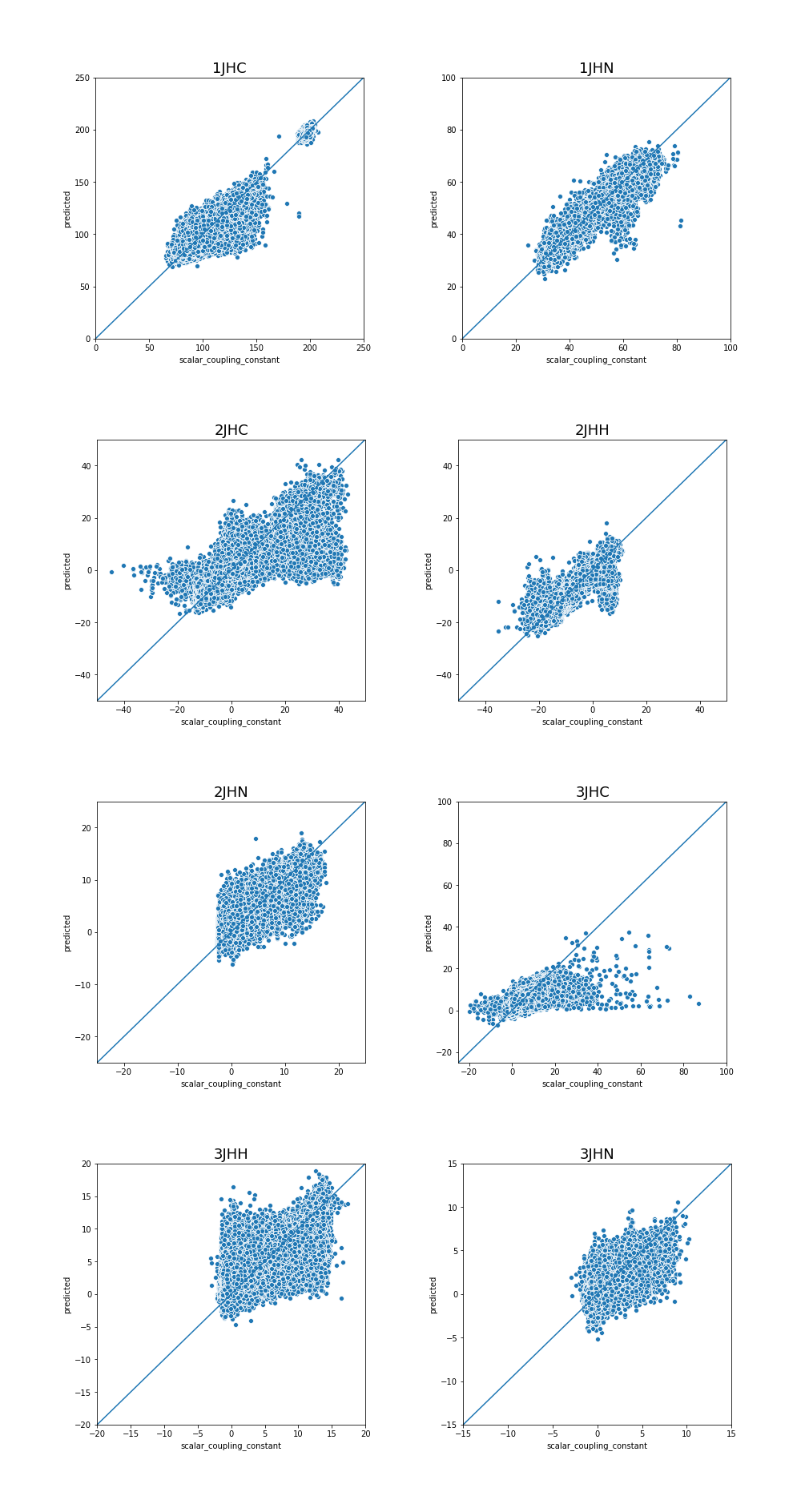
图表中显示了每个化学键类型的预测结果分布情况，数据越集中，说明我们的预测结果越一致，相比来说，效果也越好。

plot_data = pd.DataFrame(y)

plot_data.index.name = 'id'

plot_data['yhat'] = result_dict_lgb['oof']

plot_data['type'] = lbl.inverse_transform(X['type'])

def plot_oof_preds(ctype, llim, ulim):

        plt.figure(figsize=(6,6))

        sns.scatterplot(x='scalar_coupling_constant',y='yhat',

                        data=plot_data.loc[plot_data['type']==ctype,

                        ['scalar_coupling_constant', 'yhat']]);

        plt.xlim((llim, ulim))

        plt.ylim((llim, ulim))

        plt.plot([llim, ulim], [llim, ulim])

        plt.xlabel('scalar_coupling_constant')

        plt.ylabel('predicted')

        plt.title(f'{ctype}', fontsize=18)

        plt.show()

plot_oof_preds('1JHC', 0, 250)

plot_oof_preds('1JHN', 0, 100)

plot_oof_preds('2JHC', -50, 50)

plot_oof_preds('2JHH', -50, 50)

plot_oof_preds('2JHN', -25, 25)

plot_oof_preds('3JHC', -25, 100)

plot_oof_preds('3JHH', -20, 20)

plot_oof_preds('3JHN', -15, 15)

“预测分子属性”案例将在矩池云上线，感兴趣的用户可以在矩池云Demo镜像中体验。