一元回归_R相关系数_多重检验

python机器学习-乳腺癌细胞挖掘（博主亲自录制视频）https://study.163.com/course/introduction.htm?courseId=1005269003&utm_campaign=commission&utm_source=cp-400000000398149&utm_medium=share

文件夹需要两个包

normality_check.py

# -*- coding: utf-8 -*-
'''
Author：Toby
QQ：231469242，all right reversed,no commercial use
normality_check.py
正态性检验脚本

'''

import scipy
from scipy.stats import f
import numpy as np
import matplotlib.pyplot as plt
import scipy.stats as stats
# additional packages
from statsmodels.stats.diagnostic import lillifors

#正态分布测试
def check_normality(testData):
    #20<样本数<50用normal test算法检验正态分布性
    if 20<len(testData) <50:
       p_value= stats.normaltest(testData)[1]
       if p_value<0.05:
           print"use normaltest"
           print "data are not normal distributed"
           return  False
       else:
           print"use normaltest"
           print "data are normal distributed"
           return True

    #样本数小于50用Shapiro-Wilk算法检验正态分布性
    if len(testData) <50:
       p_value= stats.shapiro(testData)[1]
       if p_value<0.05:
           print "use shapiro:"
           print "data are not normal distributed"
           return  False
       else:
           print "use shapiro:"
           print "data are normal distributed"
           return True

    if 300>=len(testData) >=50:
       p_value= lillifors(testData)[1]
       if p_value<0.05:
           print "use lillifors:"
           print "data are not normal distributed"
           return  False
       else:
           print "use lillifors:"
           print "data are normal distributed"
           return True

    if len(testData) >300:
       p_value= stats.kstest(testData,'norm')[1]
       if p_value<0.05:
           print "use kstest:"
           print "data are not normal distributed"
           return  False
       else:
           print "use kstest:"
           print "data are normal distributed"
           return True

#对所有样本组进行正态性检验
def NormalTest(list_groups):
    for group in list_groups:
        #正态性检验
        status=check_normality(group)
        if status==False :
            return False

'''
group1=[2,3,7,2,6]
group2=[10,8,7,5,10]
group3=[10,13,14,13,15]
list_groups=[group1,group2,group3]
list_total=group1+group2+group3
#对所有样本组进行正态性检验
NormalTest(list_groups)
'''

correlalion_multiple.py

# -*- coding: utf-8 -*-
#斯皮尔曼等级相关（Spearman’s correlation coefficient for ranked data）
import math,pylab,scipy
import numpy as np
import scipy.stats as stats
from scipy.stats import t
from scipy.stats import f
import pandas as pd
import matplotlib.pyplot as plt
from statsmodels.stats.diagnostic import lillifors
import normality_check
import statsmodels.formula.api as sm
x=[40,42,50,55,65,78,84,100,116,125,130,140]
y=[130,150,155,140,150,154,165,170,167,180,175,185]

list_group=[x,y]
sample=len(x)
#显著性
a=0.05

#数据可视化
plt.plot(x,y,'ro')
#斯皮尔曼等级相关，非参数检验
def Spearmanr(x,y):
    print("use spearmanr,Nonparametric tests")
    #样本不一致时，发出警告
    if len(x)!=len(y):
        print ("warming,the samples are not equal!")
    r,p=stats.spearmanr(x,y)
    print("spearman r**2:",r**2)
    print("spearman p:",p)
    if sample<500 and p>0.05:
        print("when sample < 500，p has no mean（>0.05）")
        print("when sample > 500，p has mean")

#皮尔森 ，参数检验
def Pearsonr(x,y):
    print("use Pearson,parametric tests")
    r,p=stats.pearsonr(x,y)
    print("pearson r**2:",r**2)
    print("pearson p:",p)
    if sample<30:
        print("when sample <30,pearson has no mean")

#皮尔森 ，参数检验,带有详细参数
def Pearsonr_details(x,y,xLabel,yLabel,formula):
    n=len(x)
    df=n-2
    data=pd.DataFrame({yLabel:y,xLabel:x})
    result = sm.ols(formula, data).fit()
    print(result.summary())

    #模型F分布显著性分析
    print('\n')
    print("linear relation Significant test:...................................")
    #如果F检验的P值<0.05，拒绝H0，x和y无显著关系，H1成立，x和y有显著关系
    if result.f_pvalue<0.05:
        print ("P value of f test<0.05,the linear relation is right.")

    #R的显著检验
    print('\n')
    print("R significant test:...................................")
    r_square=result.rsquared
    r=math.sqrt(r_square)
    t_score=r*math.sqrt(n-2)/(math.sqrt(1-r**2))
    t_std=t.isf(a/2,df)
    if t_score<-t_std or t_score>t_std:
        print ("R is significant according to its sample size")
    else:
        print ("R is not significant")

    #残差分析
    print('\n')
    print("residual error analysis:...................................")
    states=normality_check.check_normality(result.resid)
    if states==True:
        print("the residual error are normal distributed")
    else:
        print("the residual error are not normal distributed")

    #残差偏态和峰态
    Skew = stats.skew(result.resid, bias=True)
    Kurtosis = stats.kurtosis(result.resid, fisher=False,bias=True)
    if round(Skew,1)==0:
        print("residual errors normality Skew:in middle,perfect match")
    elif  round(Skew,1)>0:
        print("residual errors normality Skew:close right")
    elif  round(Skew,1)<0:
        print("residual errors normality Skew:close left")

    if round(Kurtosis,1)==3:
        print("residual errors normality Kurtosis:in middle,perfect match")
    elif  round(Kurtosis,1)>3:
        print("residual errors normality Kurtosis:more peak")
    elif  round(Kurtosis,1)<3:
        print("residual errors normality Kurtosis:more flat")   

    #自相关分析autocorrelation
    print('\n')
    print("autocorrelation test:...................................")
    DW = np.sum( np.diff( result.resid.values )**2.0 )/ result.ssr
    if round(DW,1)==2:
        print("Durbin-Watson close to 2,there is no autocorrelation.OLS model works well")
    else:
        print("there may be autocorrelation")
    #共线性检查
    print('\n')
    print("multicollinearity test:")
    conditionNumber=result.condition_number
    if conditionNumber>30:
        print("conditionNumber>30,multicollinearity exists")
    else:
        print("conditionNumber<=30,multicollinearity not exists")

    #绘制残差图，用于方差齐性检验
    Draw_residual(list(result.resid))
'''
result.rsquared
Out[28]: 0.61510660055413524
'''

#kendalltau非参数检验
def Kendalltau(x,y):
    print("use kendalltau,Nonparametric tests")
    r,p=stats.kendalltau(x,y)
    print("kendalltau r**2:",r**2)
    print("kendalltau p:",p)

#选择模型
def R_mode(x,y,xLabel,yLabel,formula):
    #正态性检验
    Normal_result=normality_check.NormalTest(list_group)
    print ("normality result:",Normal_result)
    if len(list_group)>2:
        Kendalltau(x,y)
    if Normal_result==False:
        Spearmanr(x,y)
        Kendalltau(x,y)
    if Normal_result==True:
        Pearsonr_details(x,y,xLabel,yLabel,formula)

#调整的R方
def Adjust_Rsquare(r_square,n,k):
    adjust_rSquare=1-((1-r_square)*(n-1)*1.0/(n-k-1))
    return adjust_rSquare
'''
n=len(x)
n=10
k=1
 r_square=0.615
 Adjust_Rsquare(r_square,n,k)
Out[11]: 0.566875
'''   

#绘图
def Plot(x,y,yLabel,xLabel,Title):
    plt.plot(x,y,'ro')
    plt.ylabel(yLabel)
    plt.xlabel(xLabel)
    plt.title(Title)
    plt.show()

#绘图参数
yLabel='Alcohol'
xLabel='Tobacco'
Title='Sales in Several UK Regions'
Plot(x,y,yLabel,xLabel,Title)
formula='Alcohol ~ Tobacco'   

#绘制残点图
def Draw_residual(residual_list):
    x=[i for i in range(1,len(residual_list)+1)]
    y=residual_list
    pylab.plot(x,y,'ro')
    pylab.title("draw residual to check wrong number")

    # Pad margins so that markers don't get clipped by the axes,让点不与坐标轴重合
    pylab.margins(0.3)

    #绘制网格
    pylab.grid(True)

    pylab.show()

R_mode(x,y,xLabel,yLabel,formula)

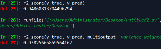
sklearn r平方计算

from sklearn.metrics import r2_score
y_true = [3, -0.5, 2, 7]
y_pred = [2.5, 0.0, 2, 8]
r2_score(y_true, y_pred)  

y_true = [[0.5, 1], [-1, 1], [7, -6]]
y_pred = [[0, 2], [-1, 2], [8, -5]]
r2_score(y_true, y_pred, multioutput='variance_weighted')

　

 https://study.163.com/provider/400000000398149/index.htm?share=2&shareId=400000000398149（ 欢迎关注博主主页，学习python视频资源，还有大量免费python经典文章）