[Scikit-learn] 1.1 Generalized Linear Models - Neural network models

本章涉及到的若干知识点（红字）；本章节是作为通往Tensorflow的前奏！

链接：https://www.zhihu.com/question/27823925/answer/38460833

首先，神经网络的最后一层，也就是输出层，是一个 Logistic Regression （或者 Softmax Regression ），也就是一个线性分类器。

那么，输入层和中间那些隐层又在干吗呢？你可以把它们看成一种特征提取的过程，就是把 Logistic Regression 的输出当作特征，然后再将它送入下一个 Logistic Regression，一层层变换。

神经网络的训练，实际上就是同时训练特征提取算法以及最后的 Logistic Regression的参数。

为什么要特征提取呢，因为 Logistic Regression 本身是一个线性分类器，所以，通过特征提取，我们可以把原本线性不可分的数据变得线性可分。

要如何训练呢，最简单的方法是（随机，Mini batch）梯度下降法（当然有更复杂的例如MATLAB里面用的是 BFGS），那要如何算梯度呢，我们通过导数的链式法则，得出一种称为 back-propagation 的方法（BP）。

最后，我们得到了一个比 Logistic Regression 复杂得多的模型，它的拟合能力很强，可以处理很多 Logistic Regression处理不了的数据，但是也更容易过拟合（ VC inequality 告诉我们，能力越大责任越大），而且损失函数不是凸的，给优化带来一些困难。

所以我们无法回答什么是“优于”，就像我们无法回答“菜刀和火箭筒哪个更好”，使用者对机器学习的理解，以及具体数据的情况，参数的选择，以及训练的方法，都对模型的效果产生很大影响。

一个建议，普通问题还是用 SVM 吧，SVM 最好用了。

 

 

 

多层感知机

---

多层多分类

Goto: http://scikit-learn.org/stable/modules/neural_networks_supervised.html

It trains using some form of gradient descent and the gradients are calculated using Backpropagation.

For classification, it minimizes the Cross-Entropy loss function, giving a vector of probability estimates  per sample .

其实就是softmax一样的道理！

举个栗子

1.17.2. Classification

"""
========================================================
Compare Stochastic learning strategies for MLPClassifier
========================================================

This example visualizes some training loss curves for different stochastic
learning strategies, including SGD and Adam. Because of time-constraints, we
use several small datasets, for which L-BFGS might be more suitable. The
general trend shown in these examples seems to carry over to larger datasets,
however.

Note that those results can be highly dependent on the value of
``learning_rate_init``.
"""

print(__doc__)
import matplotlib.pyplot as plt
from sklearn.neural_network import MLPClassifier
from sklearn.preprocessing import MinMaxScaler
from sklearn import datasets

# different learning rate schedules and momentum parameters
params = [{'solver': 'sgd', 'learning_rate': 'constant',   'momentum': 0,                               'learning_rate_init': 0.2},
          {'solver': 'sgd', 'learning_rate': 'constant',   'momentum': .9, 'nesterovs_momentum': False, 'learning_rate_init': 0.2},
          {'solver': 'sgd', 'learning_rate': 'constant',   'momentum': .9, 'nesterovs_momentum': True,  'learning_rate_init': 0.2},　　 # top one
          {'solver': 'sgd', 'learning_rate': 'invscaling', 'momentum': 0,                               'learning_rate_init': 0.2},
          {'solver': 'sgd', 'learning_rate': 'invscaling', 'momentum': .9, 'nesterovs_momentum': True,  'learning_rate_init': 0.2},
          {'solver': 'sgd', 'learning_rate': 'invscaling', 'momentum': .9, 'nesterovs_momentum': False, 'learning_rate_init': 0.2},
          {'solver': 'adam',                                                                            'learning_rate_init': 0.01}]　　# top two

labels = ["constant learning-rate", 
          "constant with momentum",
          "constant with Nesterov's momentum",
          "inv-scaling learning-rate", 
          "inv-scaling with momentum",
          "inv-scaling with Nesterov's momentum", 
          "adam"]

plot_args = [{'c': 'red',   'linestyle': '-'},
             {'c': 'green', 'linestyle': '-'},
             {'c': 'blue',  'linestyle': '-'},
             {'c': 'red',   'linestyle': '--'},
             {'c': 'green', 'linestyle': '--'},
             {'c': 'blue',  'linestyle': '--'},
             {'c': 'black', 'linestyle': '-'}]

# 重点
def plot_on_dataset(X, y, ax, name):
    # for each dataset, plot learning for each learning strategy
    print("\nlearning on dataset %s" % name)
    ax.set_title(name)
    X = MinMaxScaler().fit_transform(X)　　# 区间缩放，返回值为缩放到[0，1]区间的数据
    mlps = []
    if name == "digits":
        # digits is larger but converges fairly quickly
        max_iter = 15
    else:
        max_iter = 400

    for label, param in zip(labels, params):
        print("training: %s" % label)
        mlp = MLPClassifier(verbose=0, random_state=0, max_iter=max_iter, **param)
        mlp.fit(X, y)
        mlps.append(mlp)
        print("Training set score: %f" % mlp.score(X, y))
        print("Training set loss: %f"  % mlp.loss_)
    for mlp, label, args in zip(mlps, labels, plot_args):
            ax.plot(mlp.loss_curve_, label=label, **args)

# Start from here.
fig, axes = plt.subplots(2, 2, figsize=(15, 10))
# load / generate some toy datasets
iris      = datasets.load_iris()
digits    = datasets.load_digits()
data_sets = [(iris.data, iris.target),
             (digits.data, digits.target),
             datasets.make_circles(noise=0.2, factor=0.5, random_state=1),　　# 什么玩意？
             datasets.make_moons(noise=0.3, random_state=0)]
# 通过zip获取每一个小组的某一个名次的elem，构成一个处理集合
for ax, data, name in zip(axes.ravel(), data_sets, ['iris', 'digits', 'circles', 'moons']):
    plot_on_dataset(*data, ax=ax, name=name)

fig.legend(ax.get_lines(), labels=labels, ncol=3, loc="upper center")
plt.show()

Result:

Training set score: 0.980000
Training set loss: 0.096922
training: constant with momentum
Training set score: 0.980000
Training set loss: 0.050260
training: constant with Nesterov's momentum
Training set score: 0.980000
Training set loss: 0.050277
training: inv-scaling learning-rate
Training set score: 0.360000
Training set loss: 0.979983
training: inv-scaling with momentum
Training set score: 0.860000
Training set loss: 0.504017
training: inv-scaling with Nesterov's momentum
Training set score: 0.860000
Training set loss: 0.504760
training: adam
Training set score: 0.980000
Training set loss: 0.046248

learning on dataset digits
training: constant learning-rate
Training set score: 0.956038
Training set loss: 0.243802
training: constant with momentum
Training set score: 0.992766
Training set loss: 0.041297
training: constant with Nesterov's momentum
Training set score: 0.993879
Training set loss: 0.042898
training: inv-scaling learning-rate
Training set score: 0.638843
Training set loss: 1.855465
training: inv-scaling with momentum
Training set score: 0.912632
Training set loss: 0.290584
training: inv-scaling with Nesterov's momentum
Training set score: 0.909293
Training set loss: 0.318387
training: adam
Training set score: 0.991653
Training set loss: 0.045934

learning on dataset circles
training: constant learning-rate
Training set score: 0.830000
Training set loss: 0.681498
training: constant with momentum
Training set score: 0.940000
Training set loss: 0.163712
training: constant with Nesterov's momentum
Training set score: 0.940000
Training set loss: 0.163012
training: inv-scaling learning-rate
Training set score: 0.500000
Training set loss: 0.692855
training: inv-scaling with momentum
Training set score: 0.510000
Training set loss: 0.688376
training: inv-scaling with Nesterov's momentum
Training set score: 0.500000
Training set loss: 0.688593
training: adam
Training set score: 0.930000
Training set loss: 0.159988

learning on dataset moons
training: constant learning-rate
Training set score: 0.850000
Training set loss: 0.342245
training: constant with momentum
Training set score: 0.850000
Training set loss: 0.345580
training: constant with Nesterov's momentum
Training set score: 0.850000
Training set loss: 0.336284
training: inv-scaling learning-rate
Training set score: 0.500000
Training set loss: 0.689729
training: inv-scaling with momentum
Training set score: 0.830000
Training set loss: 0.512595
training: inv-scaling with Nesterov's momentum
Training set score: 0.830000
Training set loss: 0.513034
training: adam
Training set score: 0.850000
Training set loss: 0.334243

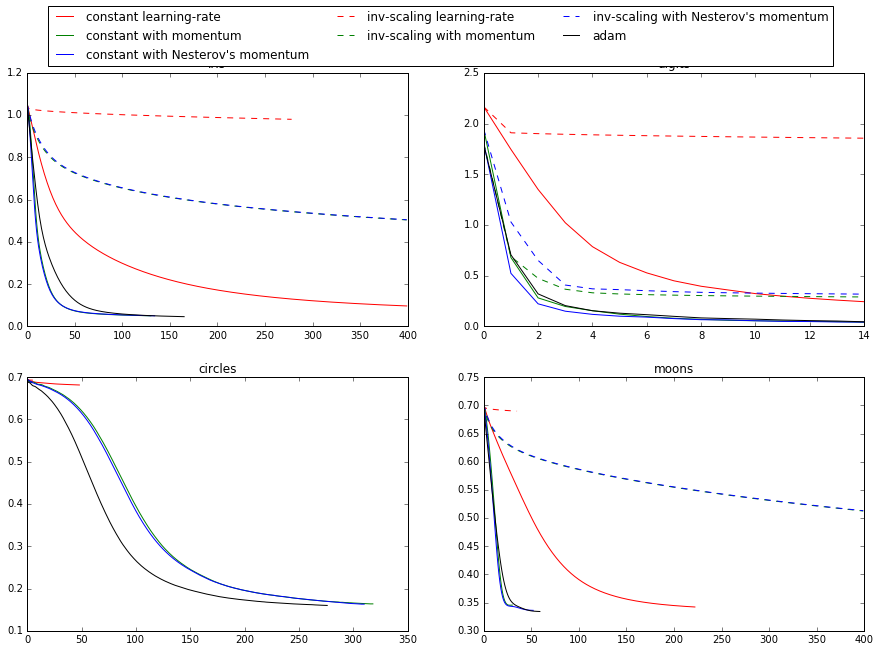
函数参数解析

多层感知机函数：

mlp = (verbose=0, random_state=0, max_iter=max_iter, **param)

【sklearn.neural_network.MLPClassifier】

Parameters:

hidden_layer_sizes : tuple, length = n_layers - 2, default (100,) The ith element represents the number of neurons in the ith hidden layer. 澄清： hidden_layer_sizes=(7,) if you want only 1 hidden layer with 7 hidden units. hidden_layer_sizes=(10,10,10) if you want 3 hidden layers with 10 hidden units each activation : {‘identity’, ‘logistic’, ‘tanh’, ‘relu’}, default ‘relu’ Activation function for the hidden layer. ‘identity’, no-op activation, useful to implement linear bottleneck, returns f(x) = x ‘logistic’,  the logistic sigmoid function, returns f(x) = 1 / (1 + exp(-x)). ‘tanh’,     the hyperbolic tan function, returns f(x) = tanh(x). ‘relu’,      the rectified linear unit function, returns f(x) = max(0, x) solver : {‘lbfgs’, ‘sgd’, ‘adam’}, default ‘adam’ The solver for weight optimization. ‘lbfgs’ is an optimizer in the family of quasi-Newton methods. ‘sgd’ refers to stochastic gradient descent. ‘adam’ refers to a stochastic gradient-based optimizer proposed by Kingma, Diederik, and Jimmy Ba Note: The default solver ‘adam’ works pretty well on relatively large datasets (with thousands of training samples or more) in terms of both training time and validation score. For small datasets, however, ‘lbfgs’ can converge faster and perform better. alpha : float, optional, default 0.0001 penalty (regularization term) parameter. batch_size : int, optional, default ‘auto’ Size of minibatches for stochastic optimizers. If the solver is ‘lbfgs’, the classifier will not use minibatch. When set to “auto”, batch_size=min(200, n_samples) learning_rate : {‘constant’, ‘invscaling’, ‘adaptive’}, default ‘constant’ Learning rate schedule for weight updates. ‘constant’ is a constant learning rate given by ‘learning_rate_init’. ‘invscaling’ gradually decreases the learning rate learning_rate_ at each time step ‘t’ using an inverse scaling exponent of ‘power_t’. effective_learning_rate = learning_rate_init / pow(t, power_t) ‘adaptive’ keeps the learning rate constant to ‘learning_rate_init’ as long as training loss keeps decreasing. Each time two consecutive epochs fail to decrease training loss by at least tol, or fail to increase validation score by at least tol if ‘early_stopping’ is on, the current learning rate is divided by 5. Only used when solver='sgd'. max_iter : int, optional, default 200 Maximum number of iterations. The solver iterates until convergence (determined by ‘tol’) or this number of iterations. random_state : int or RandomState, optional, default None State or seed for random number generator. shuffle : bool, optional, default True 多则洗牌，少则不必 Whether to shuffle samples in each iteration. Only used when solver=’sgd’ or ‘adam’. tol : float, optional, default 1e-4 Tolerance for the optimization. When the loss or score is not improving by at least tol for two consecutive iterations, unless learning_rate is set to ‘adaptive’, convergence is considered to be reached and training stops. learning_rate_init : double, optional, default 0.001 The initial learning rate used. It controls the step-size in updating the weights. Only used when solver=’sgd’ or ‘adam’. power_t : double, optional, default 0.5 The exponent for inverse scaling learning rate. It is used in updating effective learning rate when the learning_rate is set to ‘invscaling’. Only used when solver=’sgd’. verbose : bool, optional, default False Whether to print progress messages to stdout. warm_start : bool, optional, default False When set to True, reuse the solution of the previous call to fit as initialization, otherwise, just erase the previous solution. momentum : float, default 0.9 Momentum for gradient descent update. Should be between 0 and 1. Only used when solver=’sgd’. nesterovs_momentum : boolean, default True    这是什么好东东？ Whether to use Nesterov’s momentum. Only used when solver=’sgd’ and momentum > 0. early_stopping : bool, default False Whether to use early stopping to terminate training when validation score is not improving. If set to true, it will automatically set aside 10% of training data as validation and terminate training when validation score is not improving by at least tol for two consecutive epochs. Only effective when solver=’sgd’ or ‘adam’ validation_fraction : float, optional, default 0.1 The proportion of training data to set aside as validation set for early stopping. Must be between 0 and 1. Only used if early_stopping is True beta_1 : float, optional, default 0.9 Exponential decay rate for estimates of first moment vector in adam, should be in [0, 1). Only used when solver=’adam’ beta_2 : float, optional, default 0.999 Exponential decay rate for estimates of second moment vector in adam, should be in [0, 1). Only used when solver=’adam’ epsilon : float, optional, default 1e-8 Value for numerical stability in adam. Only used when solver=’adam’

参数的可视化

再来一盘例子：第一层 weight 的可视化

"""
=====================================
Visualization of MLP weights on MNIST
=====================================

Sometimes looking at the learned coefficients of a neural network can provide
insight into the learning behavior. For example if weights look unstructured,
maybe some were not used at all, or if very large coefficients exist, maybe
regularization was too low or the learning rate too high.

This example shows how to plot some of the first layer weights in a
MLPClassifier trained on the MNIST dataset.

The input data consists of 28x28 pixel handwritten digits, leading to 784
features in the dataset. Therefore the first layer weight matrix have the shape
(784, hidden_layer_sizes[0]).  We can therefore visualize a single column of
the weight matrix as a 28x28 pixel image.

To make the example run faster, we use very few hidden units, and train only
for a very short time. Training longer would result in weights with a much
smoother spatial appearance.
"""
print(__doc__)

import matplotlib.pyplot as plt
from sklearn.datasets import fetch_mldata
from sklearn.neural_network import MLPClassifier

mnist = fetch_mldata("MNIST original")
# rescale the data, use the traditional train/test split
X, y = mnist.data / 255., mnist.target
X_train, X_test = X[:60000], X[60000:]
y_train, y_test = y[:60000], y[60000:]

# mlp = MLPClassifier(hidden_layer_sizes=(100, 100), max_iter=400, alpha=1e-4,
#                     solver='sgd', verbose=10, tol=1e-4, random_state=1)
mlp = MLPClassifier(hidden_layer_sizes = (50,),
                    max_iter           = 10,
                    alpha              = 1e-4,
                    solver             = 'sgd',
                    verbose            = 10,
                    tol                = 1e-4,
                    random_state       = 1,
                    learning_rate_init = .1)

mlp.fit(X_train, y_train)
print("Training set score: %f" % mlp.score(X_train, y_train))
print("Test set score: %f" % mlp.score(X_test, y_test))

fig, axes = plt.subplots(4, 4)
# use global min / max to ensure all weights are shown on the same scale
vmin, vmax = mlp.coefs_[0].min(), mlp.coefs_[0].max()

# 根据 axes.ravel() 的大小，只画了16个
for coef, ax in zip(mlp.coefs_[0].T, axes.ravel()):
    ax.matshow(coef.reshape(28, 28), cmap=plt.cm.gray, vmin=.5 * vmin, vmax=.5 * vmax)
    ax.set_xticks(())
    ax.set_yticks(())

plt.show()

coefs的解释：

# Layer 1 --> Layer 2
len(mlp.coefs_[0])
Out[27]: 784

len(mlp.coefs_[0][0])
Out[28]: 50

784*50条边，每一条边代表一个权值。

# Layer 2 --> Layer 3
len(mlp.coefs_[1])
Out[29]: 50

len(mlp.coefs_[1][0])
Out[30]: 10

Result: 

一个方块代表一个hiden node与28*28个input node的权重分布图

End.