粒子滤波跟踪移动机器人(MATLAB Robotics System Toolbox)

　　MathWorks从MATLAB 2015a开始推出与ROS集成的Robotics System Toolbox（机器人系统工具箱），它为自主移动机器人的研发提供现成的算法和硬件接口。

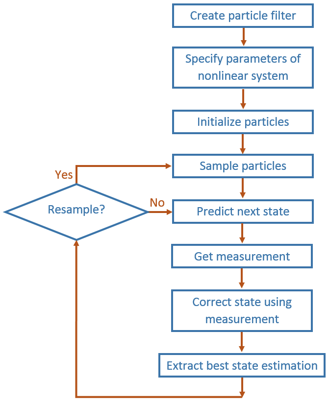
• 粒子滤波基本流程

A particle filter is a recursive, Bayesian state estimator that uses discrete particles to approximate the posterior distribution of the estimated state.

The particle filter algorithm computes the state estimate recursively and involves two steps:

• Prediction – The algorithm uses the previous state to predict the current state based on a given system model.

• Correction – The algorithm uses the current sensor measurement to correct the state estimate.

The algorithm also periodically redistributes, or resamples, the particles in the state space to match the posterior distribution of the estimated state.

The estimated state consists of all the state variables. Each particle represents a discrete state hypothesis. The set of all particles is used to help determine the final state estimate.

When using a particle filter, there is a required set of steps to create the particle filter and estimate state. The prediction and correction steps are the main iteration steps for continuously estimating state.

• 粒子滤波参数

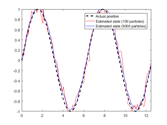
　　1. 粒子数目：The default number of particles is 1000. Unless performance is an issue, do not use fewer than 1000 particles. A higher number of particles can improve the estimate but sacrifices performance speed, because the algorithm has to process more particles. Tuning the number of particles is the best way to improve the tracking of your particle filter.

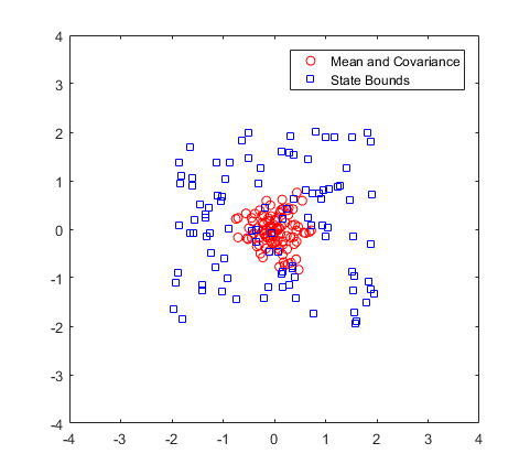
　　2. 初始位置：If you have an initial estimated state, specify it as your initial mean with a covariance relative to your system. This covariance correlates to the uncertainty of your system. The ParticleFilter object distributes particles based on your covariance around the given mean. The algorithm uses this distribution of particles to get the best estimation of state, so an accurate initialization of particles helps to converge to the best state estimation quickly. If an initial state is unknown, you can evenly distribute your particles across a given state bounds. The state bounds are the limits of your state. For example, when estimating the position of a robot, the state bounds are limited to the environment that the robot can actually inhabit. In general, an even distribution of particles is a less efficient way to initialize particles to improve the speed of convergence. The plot shows how the mean and covariance specification can cluster particles much more effectively in a space rather than specifying the full state bounds.

　　3. 状态转移函数：The state transition function, StateTransitionFcn, of a particle filter helps to evolve the particles to the next state. It is used during the prediction step of the Particle Filter Workflow. In the ParticleFilter object, it is specified as a callback function that takes the previous particles, and any other necessary parameters, and outputs the predicted location. By default, the state transition function assumes a Gaussian motion model with constant velocities. The function uses a Gaussian distribution to determine the position of the particles in the next time step. For your application, it is important to have a state transition function that accurately describes how you expect the system to behave. To accurately evolve all the particles, you must develop and implement a motion model for your system. If particles are not distributed around the next state, the ParticleFilter object does not find an accurate estimate. Therefore, it is important to understand how your system can behave so that you can track it accurately.

　　4. Measurement Likelihood Function：After predicting the next state, you can use measurements from sensors to correct your predicted state. By specifying a MeasurementLikelihoodFcn in the ParticleFilter object, you can correct your predicted particles using the correct function. This measurement likelihood function, by definition, gives a weight for the state hypotheses (your particles) based on a given measurement. Essentially, it gives you the likelihood that the observed measurement actually matches what each particle observes. This likelihood is used as a weight on the predicted particles to help with correcting them and getting the best estimation

　　5. 状态估计方法：The final step of the particle filter workflow is the selection of a single state estimate. The particles and their weights sampled across the distribution are used to give the best estimation of the actual state. However, you can use the particles information to get a single state estimate in multiple ways. With the ParticleFilter object, you can either choose the best estimate based on the particle with the highest weight or take a mean of all the particles. Specify the estimtation method in the StateEstimationMethod property as either'mean'(default) or 'maxweight'.

•  Track a Robot Using Particle Filter

　　A remote-controlled robot is being tracked in the outdoor environment. The robot pose measurement is now provided by an on-board GPS, which is noisy. We also know the motion commands sent to the robot, but the robot will not execute the exact commanded motion due to mechanical part slacks and/or model inaccuracy. This example will show how to use robotics.ParticleFilter to reduce the effects of noise in the measurement data and get a more accurate estimation of the pose of the robot. The kinematic model of a car-like robot is described by the following non-linear system.

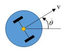
　　移动机器人可以控制线速度和转向角速度，其位置和姿态(, , )可以通过GPS定位系统或光学捕捉系统等手段获取。由于存在噪声因此测量和控制都存在一定误差（There will be some difference between the commanded motion and the actual motion of the robot）。设系统状态变量为 [ , , , , ,  ].

　　机器人转向时可以看作绕着轴线上的瞬时曲率中心（The point that the robot rotates about is known as the ICC - Instantaneous Center of Curvature）旋转，曲率半径为R。假设两轮间距为L，左右轮速度分别为v_l、v_r，则有：

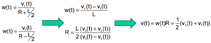
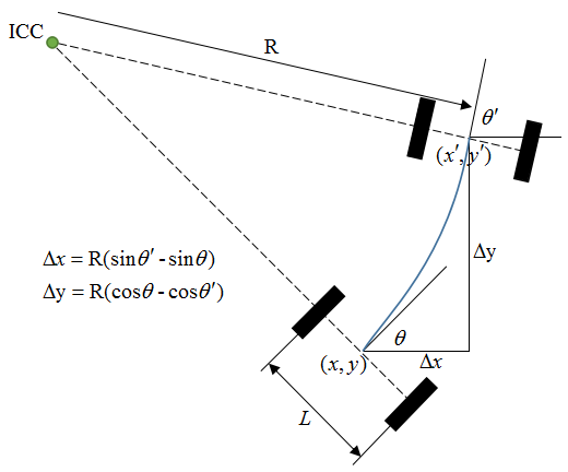
　　根据运动学模型，可以得到系统状态方程，状态转移函数的实现如下：

function predictParticles = BotStateTransition(pf, prevParticles, dT, u)
   thetas = prevParticles(:,3);
   w = u(2);
   v = u(1);
   n = length(prevParticles);

   % Generate velocity samples
   sd1 = 0.3;  % sd1 represents the uncertainty in the linear velocity
   sd2 = 1.5;  % sd2 represents the uncertainty in the angular velocity
   sd3 = 0.02; % sd3 is an additional perturbation on the orientation
   vh = v + (sd1)^2*randn(n,1);
   wh = w + (sd2)^2*randn(n,1);
   gamma = (sd3)^2*randn(n,1);

   % Add a small number to prevent div/0 error
   wh(abs(wh)<1e-19) = 1e-19;

   % State Transition
   predictParticles(:,1) = prevParticles(:,1) - (vh./wh).*sin(thetas) + (vh./wh).*sin(thetas + wh*dT);
   predictParticles(:,2) = prevParticles(:,2) + (vh./wh).*cos(thetas) - (vh./wh).*cos(thetas + wh*dT);
   predictParticles(:,3) = prevParticles(:,3) + wh*dT + gamma*dT;
   predictParticles(:,4) = (- (vh./wh).*sin(thetas) + (vh./wh).*sin(thetas + wh*dT))/dT;
   predictParticles(:,5) = ( (vh./wh).*cos(thetas) - (vh./wh).*cos(thetas + wh*dT))/dT;
   predictParticles(:,6) = wh + gamma;
end

　　然后要实现Measurement Likelihood Function，它会根据预测值与测量值之间的误差大小来计算每个粒子的权值。与观测值越接近的粒子权值越大，反之越小。这个例子中粒子是一个N×6的矩阵（N为粒子数目），测量值是1×3的向量。函数的实现如下：

function  likelihood = BotMeasurementLikelihood(pf, predictParticles, measurement)
   % The measurement contains all state variables
   predictMeasurement = predictParticles;

   % Calculate observed error between predicted and actual measurement
   measurementError = bsxfun(@minus, predictMeasurement(:,1:3), measurement); % applies an element-by-element binary operation to arrays
   measurementErrorNorm = sqrt(sum(measurementError.^2, 2));

   % Normal-distributed noise of measurement
   % Assuming measurements on all three pose components have the same error distribution
   measurementNoise = eye(3);

   % Convert error norms into likelihood measure.
   % Evaluate the PDF of the multivariate normal distribution
   likelihood = 1/sqrt((2*pi).^3 * det(measurementNoise)) * exp(-0.5 * measurementErrorNorm);
end

　　下面是整个Workflow的代码，其中利用了MATLAB自带的函数ExampleHelperCarBot来创建移动机器人（该模型与汽车类似，前面两轮驱动和转向，本例与该模型存在一定的差异），并利用相关的函数来绘制跟踪图像。注意当机器人运动到有屋顶的区域时，由于遮挡GPS信号丢失，返回的测量值为空。

%% Initialize Robot
rng('default'); % for repeatable result
dt = 0.05;      % Time step for simulation of the robot
initialPose = [0  0  0  0]';
carbot = ExampleHelperCarBot(initialPose, dt);

%% Set up the Particle Filter
pf = robotics.ParticleFilter;

initialize(pf, 5000, [initialPose(1:3)', 0, 0, 0], eye(6), 'CircularVariables',[0 0 1 0 0 0]);
pf.StateEstimationMethod = 'mean';
pf.ResamplingMethod = 'systematic';

% StateTransitionFcn defines how particles evolve without measurement
pf.StateTransitionFcn = @BotStateTransition;

% MeasurementLikelihoodFcn defines how measurement affect the our estimation
pf.MeasurementLikelihoodFcn = @BotMeasurementLikelihood;

% Last best estimation for x, y and theta
lastBestGuess = [0 0 0];

%% Main Loop
% Run loop at 20 Hz for 20 seconds
r = robotics.Rate(1/dt); % The Rate object enables you to run a loop at a fixed frequency
reset(r);                % Reset the fixed-rate object

% Reset simulation time
 simulationTime = 0;

while simulationTime < 20 % if time is not up

　　% Generate motion command that is to be sent to the robot
　　% NOTE there will be some discrepancy between the commanded motion and the motion actually executed by the robot.
　　uCmd(1) = 0.7*abs(sin(simulationTime)) + 0.1; % linear velocity
　　uCmd(2) = 0.08*cos(simulationTime);           % angular velocity

　　drive(carbot, uCmd); % Move the robot forward contaminate commanded motion with noise

　　% Predict the carbot pose based on the motion model
　　[statePred, covPred] = predict(pf, dt, uCmd);

　 % Get GPS reading
　 % The GPS reading is just simulated by adding Gaussian Noise to the truth data.
　 % When the robot is in the roofed area, the GPS reading will not be available, the measurement will return an empty matrix.
   measurement = exampleHelperCarBotGetGPSReading(carbot); 

   % If measurement is available, then call correct, otherwise just use predicted result
   if ~isempty(measurement)
       [stateCorrected, covCorrected] = correct(pf, measurement');
   else
       stateCorrected = statePred;
       covCorrected = covPred;
   end

   lastBestGuess = stateCorrected(1:3);

   % Update plot
   if ~isempty(get(groot,'CurrentFigure')) % if figure is not prematurely killed
       updatePlot(carbot, pf, lastBestGuess, simulationTime);
   else
       break
   end

   waitfor(r);

   % Update simulation time
   simulationTime = simulationTime + dt;
end

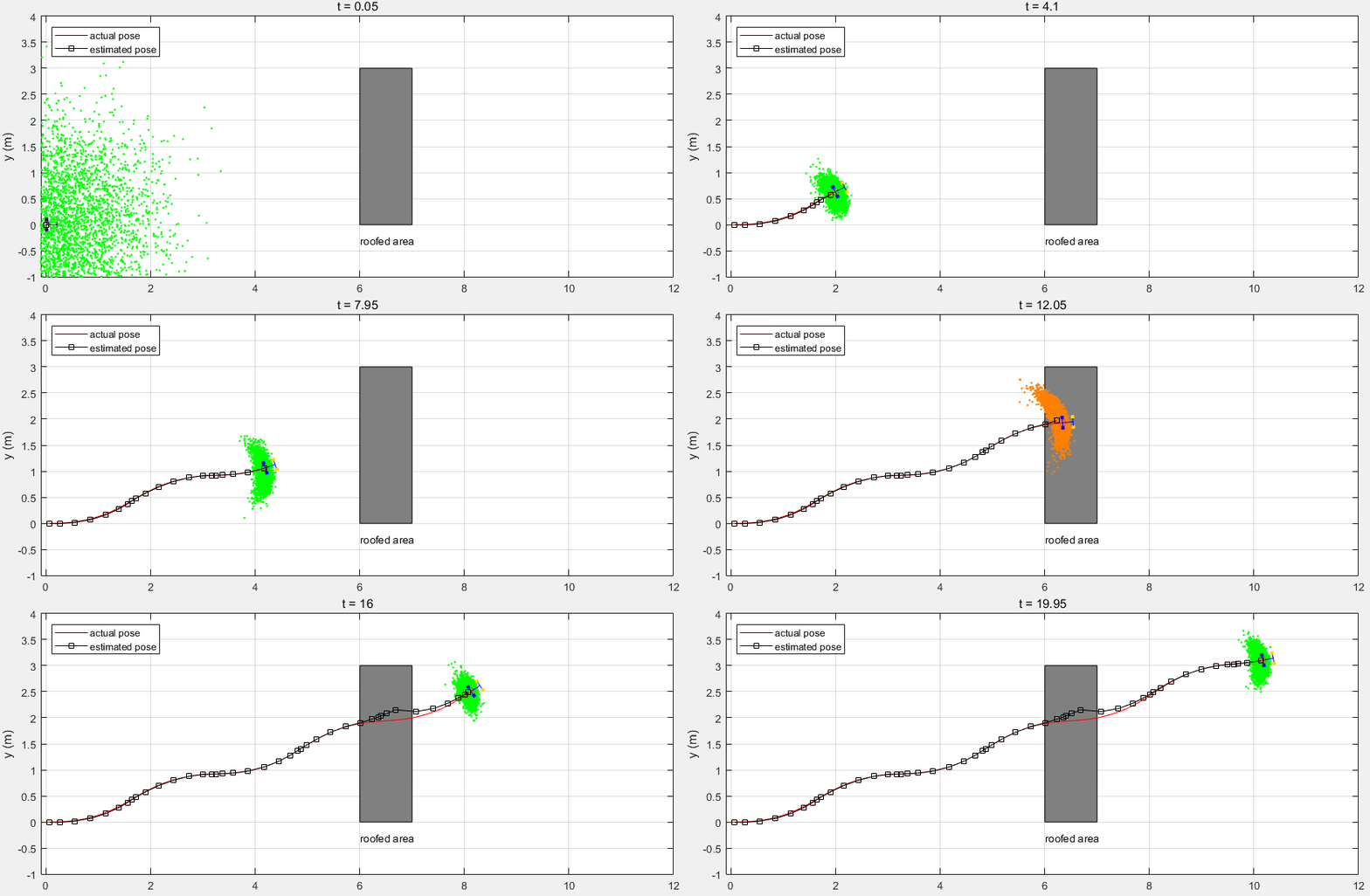
　　可以看到在有屋顶的区域，预测值与机器人真实位置出现了较大的偏差。在机器人走出该区域后，接收到GPS测量信号对预测值进行校正，得到的估计值又收敛到真实位置。

参考：

Particle Filter Workflow

Particle Filter Parameters

Track a Car-Like Robot Using Particle Filter

Localize TurtleBot Using Monte Carlo Localization

机器人粒子滤波定位（蒙特卡罗定位）

Kalman-and-Bayesian-Filters-in-Python