ADADELTA: AN ADAPTIVE LEARNING RATE METHOD

目录

• 引
• 主要内容
• 算法
• ADADELTA 代码

引

这篇论文比较短，先看了这篇，本来应该先把ADAGRAD看了的。普通的基于梯度下降的方法，普遍依赖于步长，起始点的选择，所以，受ADAGRAD的启发，作者提出了一种ADADELTA的方法。

\[\Delta x_t = -\frac{\mathrm{RMS}[\Delta x]_{t-1}}{\mathrm{RMS}[g]_t}g_t
\]

其中\(g_t=\frac{\partial f(x_t)}{\partial x_t}\)，所以下一步迭代就是:

\[x_{t+1} = x_t + \Delta x_t
\]

主要内容

ADAGRAD方法：

\[\Delta x_t = -\frac{\eta}{\sqrt{\sum_{\tau=1}^t g_{\tau}^2}}g_t
\]

也就是，步长与之前所有的梯度有关，显然这个步长是会逐渐减少的。但是这个缺点也很明显，如果起始点的梯度很大，那么就会导致后续步长很小，而一开始的梯度很小，就会导致后续步长很大，产生振荡，有些怪怪的。

而ADADELTA希望只关心一部分的梯度，比如

\[\sqrt{\sum_{\tau=t-k}^tg_{\tau}^2}
\]

但是这么做，每次迭代都必须记录\(k\)个梯度，这显得不怎么效率，于是，作者相处了一个法子：

\[E[g^2]_t = \rho E[g^2]_{t-1} + (1-\rho)g_t^2
\]

可以看到，对于\(g_1\)，\(t+1\)步之后其影响为：\(\rho^t(1-\rho) g_1\),对整个迭代造成的影响是一个等比序列：

\[(1-\rho), \rho (1-\rho), \ldots, \rho^t(1-\rho)
\]

最后趋向于：

\[1-\rho^{t+1} \rightarrow1
\]

这么做就俩劝其美啦。

记：

\[\mathrm{RMS}[g]_t = \sqrt{E[g^2]_t + \epsilon}
\]

其中\(\epsilon\)是为了让除法有意义而添加的小量。

所以

\[\Delta x_t = -\frac{\eta}{\mathrm{RMS}[g]_t}g_t
\]

这还不是最终版本，另一个启发决定了\(\eta\)的选择。

我们知道，很多问题是有实际含义的，\(x\)可能是有单位的，比如是米，天等，所以，一个很自然的期望是，\(\Delta x\)的单位和\(x\)是保持一致的。但是：

\[\mathrm{units \: of \:}\Delta x \propto \mathrm{units \: of \:} g \propto \frac{\partial f}{\partial x}\propto \frac{1}{\mathrm{units \: of \:} x}
\]

也就是说\(\Delta x\)的步长单位和梯度单位是一致的，就像是\(l=vt\)，\(\Delta t\)的步长单位是\(m/s\)，是时间单位的倒数。

而利用二阶导数迭代步长就符合单位一致(如Newton方法)：

\[\Delta x \propto H^{-1} g \propto \frac{\frac{\partial f}{\partial x}}{\frac{\partial^2 f}{\partial x^2}} \propto \mathrm{units \: of \:} x
\]

其中\(H\)为Hessian矩阵。

又注意到：

\[\Delta x = \frac{\frac{\partial f}{\partial x}}{\frac{\partial^2 f}{\partial x^2}} \Rightarrow \frac{1}{\frac{\partial^2 f}{\partial x^2}} = \frac{\Delta x}{\frac{\partial f}{\partial x}}
\]

于是，完全体的ADADELTA方法变为如下：

\[\Delta x_t = -\frac{\mathrm{RMS}[\Delta x]_{t-1}}{\mathrm{RMS}[g]_t}g_t
\]

分子式\(t-1\)的原因式\(\Delta x_t\)压根不知道，所木有办法，就将就一下。

算法

完整的算法如下：

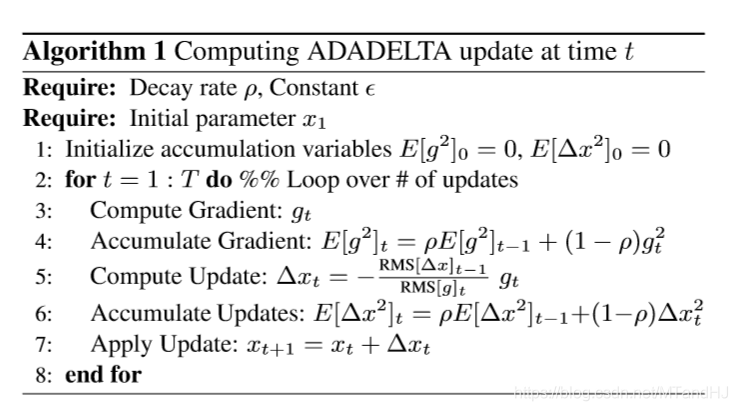
需要注意一点的是，在实际实验中，我们设置\(E[\Delta x^2]_0=1\)而不是如算法中所说的0。因为，如果设置为0，那么意味着第一步只进行相当微小的迭代，所以之后也都是微小的迭代。或许作者是将\(\epsilon\)设置为\(1\)?而不是一个小量？

ADADELTA 代码

import numpy as np
import matplotlib.pyplot as plt

这次用比较怪一点的方式来写，首先，创建一个类，用来存放函数\(f\)和梯度\(g\)

class ADADELTA:
    def __init__(self, function, gradient, rho=0.7):
        assert hasattr(function, "__call__"), "Invalid function"
        assert hasattr(gradient, "__call__"), "Invalid gradient"
        assert 0 < rho < 1, "Invalid rho"
        self.__function = function
        self.__gradient = gradient
        self.rho = rho
        self.acc_gradient = 0 #初始化accumulate gradient
        self.acc_updates = 1 #初始化accumulate updates
        self.progress = []

    @property
    def function(self):
        return self.__function

    @property
    def gradient(self):
        return self.__gradient

    def reset(self):
        self.acc_gradient = 0 #初始化accumulate gradient
        self.acc_updates = 1 #初始化accumulate updates
        self.progress = []

计算累计梯度

\[E[g^2]_t = \rho E[g^2]_{t-1} + (1-\rho)g_t^2
\]

def accumulate_gradient(self, gt):
    self.acc_gradient = self.rho * self.acc_gradient \
                            + (1 - self.rho) * gt ** 2
    return self.acc_gradient
ADADELTA.accumulate_gradient = accumulate_gradient

更新\(E[\Delta x]_t\)

\[E[\Delta x^2]_t = \rho E[\Delta x^2]_{t-1} + (1-\rho)\Delta x_t^2
\]

def accumulate_updates(self, deltax):
    self.acc_updates = self.rho * self.acc_updates \
                        + (1 - self.rho) * deltax ** 2
    return self.acc_updates
ADADELTA.accumulate_updates = accumulate_updates

计算更新步长:

\[\Delta x_t = -\frac{\mathrm{RMS}[\Delta x]_{t-1}}{\mathrm{RMS}[g]_t}g_t
\]

def step(self, x, smoothingterm=1e-8):
    gt = self.gradient(x)
    self.accumulate_gradient(gt)
    RMS_gt = np.sqrt(self.acc_gradient + smoothingterm)
    RMS_up = np.sqrt(self.acc_updates + smoothingterm)
    deltax = -RMS_up / RMS_gt * gt
    self.accumulate_updates(deltax)
    return x + deltax
ADADELTA.step = step

进行t步

def process(self, startx, t, smoothingterm=1e-8):
    x = startx
    for i in range(t):
        self.progress.append(x)
        x = self.step(x, smoothingterm)
    return self.progress
ADADELTA.process = process

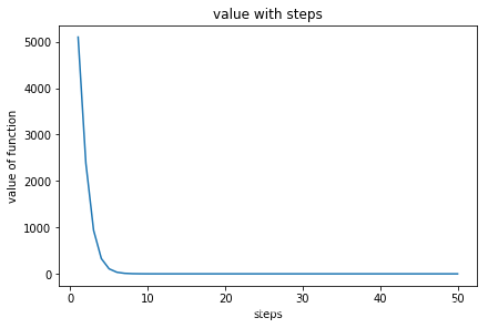
可视化

def plot(self):
    x = np.arange(1, len(self.progress) + 1)
    y = np.array([
        self.function(item) for item in self.progress
    ])
    fig, ax = plt.subplots(constrained_layout=True)
    ax.plot(x, y)
    ax.set_xlabel("steps")
    ax.set_ylabel("value of function")
    ax.set_title("value with steps")
    plt.show()
ADADELTA.plot = plot

def function(x):
    return x[0] ** 2 + 50 * x[1] ** 2

def gradient(x):
    return 2 * x[0] + 100 * x[1]

test = ADADELTA(function, gradient, 0.9)
test.reset()
startx = np.array([10, 10])
test.process(startx, 50)
test.plot()