（六）6.8 Neurons Networks implements of PCA ZCA and whitening

PCA

给定一组二维数据，每列十一组样本，共45个样本点

-6.7644914e-01  -6.3089308e-01  -4.8915202e-01 ...

-4.4722050e-01  -7.4778067e-01  -3.9074344e-01 ...

可以表示为如下形式：

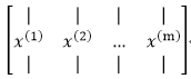
本例子中的的x⁽ⁱ⁾为2维向量，整个数据集X为2*m的矩阵，矩阵的每一列代表一个数据，该矩阵的转置X' 为一个m*2的矩阵：

假设如上数据为归一化均值后的数据(注意这里省略了方差归一化)，则数据的协方差矩阵Σ为 1/m(X*X')，Σ为一个2*2的矩阵：

对该对称矩阵对角线化：

这是对于2维情况，若对于n维，会得到一组n维的新基：

，且U的转置：

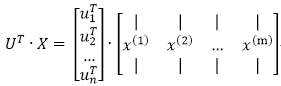
原数据在U上的投影为用U^T*X表示即可：

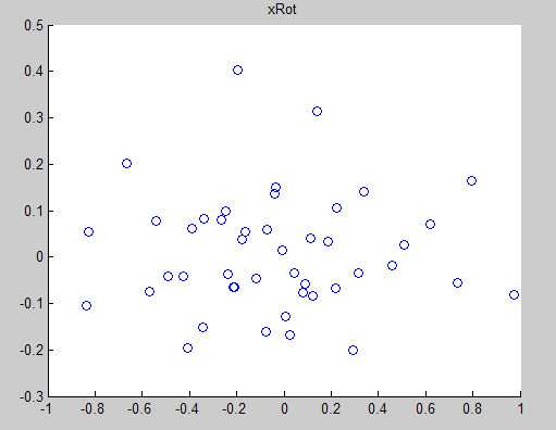
对于二维数据，U^T为2*2的矩阵，U^T*X会得到2*m的新矩阵，即原数据在新基下的表示X_ROT，原来的数据映射到这组新基上，便得到可一组在各个维度上不相关的数据，取k<n,把数据映射到上，便完成的降维过程，下图为X_ROT：

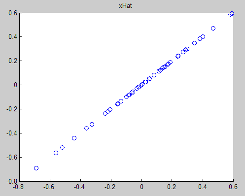
对基变换后的数据还可以进行还原，比如得到了原始数据  的低维“压缩”表征量  ， 反过来，如果给定  ，我们应如何还原原始数据  呢？  的基为要转换回来，只需  即可。进一步，我们把  看作将  的最后  个元素被置0所得的近似表示，因此如果给定  ，可以通过在其末尾添加  个0来得到对  的近似，最后，左乘  便可近似还原出原数据  。具体来说，计算如下：

下图为还原后的数据：

下面来看白化，白化就是先对数据进行基变换，但是并不进行降维，且对变化后的数据，每一个维度上都除以其标准差，来达到归一化均值方差的目的。另外值得一提的一段话是：

感觉除了层数和每层隐节点的个数，也没啥好调的。其它参数，近两年论文基本都用同样的参数设定：迭代几十到几百epoch。sgd，mini batch size从几十到几百皆可。步长0.1，可手动收缩，weight decay取0.005，momentum取0.9。dropout加relu。weight用高斯分布初始化，bias全初始化为0。最后记得输入特征和预测目标都做好归一化。做完这些你的神经网络就应该跑出基本靠谱的结果，否则反省一下自己的人品。

对于ZCA，直接在PCAwhite 的基础上左成特征矩阵U即可，

matlab代码：

close all

%%================================================================
%% Step 0: Load data
%  We have provided the code to load data from pcaData.txt into x.
%  x is a 2 * 45 matrix, where the kth column x(:,k) corresponds to
%  the kth data point.Here we provide the code to load natural image data into x.
%  You do not need to change the code below.

x = load('pcaData.txt','-ascii');
figure(1);
scatter(x(1, :), x(2, :));
title('Raw data');

%%================================================================
%% Step 1a: Implement PCA to obtain U
%  Implement PCA to obtain the rotation matrix U, which is the eigenbasis
%  sigma. 

% -------------------- YOUR CODE HERE --------------------
u = zeros(size(x, 1)); % You need to compute this
[n m] = size(x);
p = mean(x,2)；%按行求均值，p为一个2维列向量
%x = x-repmat(p,1,m);%预处理，均值为0
sigma = (1.0/m)*x*x';%协方差矩阵
[u s v] = svd(sigma);%奇异值分解得到特征值与特征向量

% --------------------------------------------------------
hold on
plot([0 u(1,1)], [0 u(2,1)]);%画第一条线
plot([0 u(1,2)], [0 u(2,2)]);%第二条线
scatter(x(1, :), x(2, :));
hold off

%%================================================================
%% Step 1b: Compute xRot, the projection on to the eigenbasis
%  Now, compute xRot by projecting the data on to the basis defined
%  by U. Visualize the points by performing a scatter plot.

% -------------------- YOUR CODE HERE --------------------
xRot = zeros(size(x)); %  初始化一个基变换后的数据
xRot = u'*x;    %做基变换

% -------------------------------------------------------- 

% Visualise the covariance matrix. You should see a line across the
% diagonal against a blue background.
figure(2);
scatter(xRot(1, :), xRot(2, :));
title('xRot');

%%================================================================
%% Step 2: Reduce the number of dimensions from 2 to 1.
%  Compute xRot again (this time projecting to 1 dimension).
%  Then, compute xHat by projecting the xRot back onto the original axes
%  to see the effect of dimension reduction

% 用投影后的数据还原原始数据
k = 1; % Use k = 1 and project the data onto the first eigenbasis
xHat = zeros(size(x)); % 还原原始数据
%[u(:,1),zeros(n,1)]'*x 代表原数据在新基上的前K维的投影，之后的维度为0
%对降维后的数据进行还原：u * xRot = Xhat，Xhat为还原后的数据
xHat = u*([u(:,1),zeros(n,1)]'*x);%n代表数据的维度

% --------------------------------------------------------
figure(3);
scatter(xHat(1, :), xHat(2, :));
title('xHat');

%%================================================================
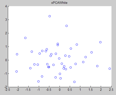
%% Step 3: PCA Whitening
%  Complute xPCAWhite and plot the results.

epsilon = 1e-5;
% -------------------- YOUR CODE HERE --------------------
xPCAWhite = zeros(size(x)); % You need to compute this
% s为对角阵，diag(s)会返回s主对角线元素组成的列向量
% diag(1./sqrt(diag(s)+epsilon))会返回一个对角阵，
% 对角线元素为  ->  1./sqrt(diag(s)+epsilon
% 变换后的数据为 ： Xrot = u'*x
%这样做对应于Xrot的数据再每个维度除以其标准差
xPCAWhite = diag(1./sqrt(diag(s)+epsilon))*u'*x;

% --------------------------------------------------------
figure(4);
scatter(xPCAWhite(1, :), xPCAWhite(2, :));
title('xPCAWhite');

%%================================================================
%% Step 3: ZCA Whitening
%  Complute xZCAWhite and plot the results.

% -------------------- YOUR CODE HERE --------------------
xZCAWhite = zeros(size(x)); % You need to compute this
xZCAWhite = u*diag(1./sqrt(diag(s)+epsilon))*u'*x;

% --------------------------------------------------------
figure(5);
scatter(xZCAWhite(1, :), xZCAWhite(2, :));
title('xZCAWhite');

%% Congratulations! When you have reached this point, you are done!
%  You can now move onto the next PCA exercise. :)

PCA与Whitening与ZCA的一个小实验：参考自http://deeplearning.stanford.edu/wiki/index.php/Exercise:PCA_and_Whitening

%%================================================================
%% Step 0a: 加载数据
% 随机采样10000张图片放入到矩阵x里.
%  x 是一个 144 * 10000 的矩阵，该矩阵的第 k列 x(:, k) 对应第k张图片
 
x = sampleIMAGESRAW();
figure('name','Raw images');
randsel = randi(size(x,2),200,1); % A random selection of samples for visualization
display_network(x(:,randsel));
 
%%================================================================
%% Step 0b: 0-均值（Zero-mean）这些数据 (按行)
%  You can make use of the mean and repmat/bsxfun functions.
[n m] = size(x);
p = mean(x,1);
x = x - repmat(p,1,m);
%%================================================================
%% Step 1a: Implement PCA to obtain xRot
%  Implement PCA to obtain xRot, the matrix in which the data is expressed
%  with respect to the eigenbasis of sigma, which is the matrix U.
 
xRot = zeros(size(x)); % 新基下的数据
sigma =(1.0/m)*x*x';
[u s v] = svd(sigma);
XRot = u'*x;
 
%%================================================================
%% Step 1b: Check your implementation of PCA
% 新基U下的数据的协方差矩阵是对角阵，只在主对角线上不为0
%  Write code to compute the covariance matrix, covar.
%  When visualised as an image, you should see a straight line across the
%  diagonal (non-zero entries) against a blue background (zero entries).
 
% -------------------- YOUR CODE HERE --------------------
covar = zeros(size(x, 1)); % You need to compute this
covar = (1./m)*xRot*xRot'; %新基下数据的均值仍然为0，直接计算covariance
 
% Visualise the covariance matrix. You should see a line across the
% diagonal against a blue background.
figure('name','Visualisation of covariance matrix');
imagesc(covar);
 
%%================================================================
%% Step 2: Find k, the number of components to retain
%  Write code to determine k, the number of components to retain in order
%  to retain at least 99% of the variance.
%  保留99%的方差比
 
% -------------------- YOUR CODE HERE --------------------
k = 0; % Set k accordingly
for i = i,n:
lambd = diag(s)%对角线元素组成的列向量
% 通过循环找到99%的方差百分比的k值
for k = 1:n
    if sum(lambd(1:k))/sum(lambd)<0.99
        continue;
end
%下面是另一种k的求法
%其中cumsum(ss)求出的是一个累积向量，也就是说ss向量值的累加值
%并且(cumsum(ss)/sum(ss))<=0.99是一个向量，值为0或者1的向量，为1表示满足那个条件
%k = length(ss((cumsum(ss)/sum(ss))<=0.99));
 
%%================================================================
%% Step 3: Implement PCA with dimension reduction
%  Now that you have found k, you can reduce the dimension of the data by
%  discarding the remaining dimensions. In this way, you can represent the
%  data in k dimensions instead of the original 144, which will save you
%  computational time when running learning algorithms on the reduced
%  representation.
%
%  Following the dimension reduction, invert the PCA transformation to produce
%  the matrix xHat, the dimension-reduced data with respect to the original basis.
%  Visualise the data and compare it to the raw data. You will observe that
%  there is little loss due to throwing away the principal components that
%  correspond to dimensions with low variation.
 
% -------------------- YOUR CODE HERE --------------------
xHat = zeros(size(x));  % You need to compute this
%把x映射到U的前k个基上 u(:,1:k)'*x作为Xrot'，Xrot'为k*m维的
%补全整个Xrot'中k到n维的元素为0，然后左乘U变回到原来的基下得到Xhat
% 首先为了降维做一个基变换，降维后要还原到原来的坐标系下，还原后为
%对应的降维后的原始数据
 
xHat = u*[u(:,1:k)'*x;zeros(n-k,m)];
 
% Visualise the data, and compare it to the raw data
% You should observe that the raw and processed data are of comparable quality.
% For comparison, you may wish to generate a PCA reduced image which
% retains only 90% of the variance.
 
figure('name',['PCA processed images ',sprintf('(%d / %d dimensions)', k, size(x, 1)),'']);
display_network(xHat(:,randsel));
figure('name','Raw images');
display_network(x(:,randsel));
 
%%================================================================
%% Step 4a: Implement PCA with whitening and regularisation
%  Implement PCA with whitening and regularisation to produce the matrix
%  xPCAWhite.
 
epsilon = 0.1;
xPCAWhite = zeros(size(x));
 
% 白化处理
% xRot = u' * x 为白化后的数据
xPCAWhite = diag(1./sqrt(diag(s) + epsilon))* u' * x;
figure('name','PCA whitened images'); display_network(xPCAWhite(:,randsel));
%%================================================================ %%
 Step 4b: Check your implementation of PCA whitening
 % Check your implementation of PCA whitening with and without regularisation.
% PCA whitening without regularisation results a covariance matrix
% that is equal to the identity matrix. PCA whitening with regularisation
% results in a covariance matrix with diagonal entries starting close to
% 1 and gradually becoming smaller. We will verify these properties here.
% Write code to compute the covariance matrix, covar.
%  Without regularisation (set epsilon to 0 or close to 0),
% when visualised as an image, you should see a red line across the
% diagonal (one entries) against a blue background (zero entries).
% With regularisation, you should see a red line that slowly turns
% blue across the diagonal, corresponding to the one entries slowly
% becoming smaller.
% -------------------- YOUR CODE HERE --------------------
% Visualise the covariance matrix. You should see a red line across the
% diagonal against a blue background. figure('name','Visualisation of covariance matrix'); imagesc(covar);
%%================================================================ %
% Step 5: Implement ZCA whitening % Now implement ZCA whitening to produce the matrix xZCAWhite.
% Visualise the data and compare it to the raw data. You should observe
% that whitening results in, among other things, enhanced edges.
xZCAWhite = zeros(size(x));
% ZCA处理
 xZCAWhite = u*xPCAWhite;
% Visualise the data, and compare it to the raw data.
% You should observe that the whitened images have enhanced edges.
figure('name','ZCA whitened images');
display_network(xZCAWhite(:,randsel)); figure('name','Raw images'); display_network(x(:,randsel));

　　参考：

http://www.cnblogs.com/tornadomeet/archive/2013/03/21/2973231.html

UFLDL