无监督学习 Kmeans

无监督学习

自动对输入数据进行分类或者分群

优点：

算法不受监督信息（偏见）的约束，可能考虑到新的信息

不需要标签数据，极大程度扩大数据样本

Kmeans 聚类

根据数据与中心点距离划分类别

基于类别数据更新中心点

重复过程直到收敛

特点：实现简单、收敛快；需要指定类别数量（需要告诉计算机要分成几类）

1. 选择聚类的个数
2. 确定聚类中心
3. 根据点到聚类中心聚类确定各个点所属类别
4. 更具各个类别数据更新聚类中心
5. 重复以上步骤直到收敛（中心点不再变化）

均值漂移聚类 Meanshift

在中心点一定区域检索数据点

更新中心

重复流程到中心点稳定

DBSCAN算法(基于密度的空间聚类算法)

基于区域点密度筛选有效数据

基于有效数据向周边扩张，直到没有新点加入

特点：过滤噪音数据；不需要人为选择类别数量；数据密度不同时影响结果

KNN K邻近分类监督学习

给定一个训练数据集，对新的输入实例，在训练数据集中找到与该实例最邻近的K个实例，这K个实例的多数属于某个类， 就把该输入实例分类到这个类中。

参考链接

https://blog.csdn.net/weixin_46344368/article/details/106036451?spm=1001.2014.3001.5502

code

#加载数据并预览
import pandas as pd
import numpy as np
data = pd.read_csv('data.csv')
data.head()
#定义X和y
X = data.drop(['labels'],axis=1)
y = data.loc[:,'labels']
y.head()#预览
pd.value_counts(y) #查看类别数(这里有0，1，2三个类别)以及每个类别对应的样本数
#导入数据以及数据可视化
%matplotlib inline
from matplotlib import pyplot as plt
fig1 = plt.figure()
plt.scatter(X.loc[:,'V1'],X.loc[:,'V2'])
plt.title("un-labled data")
plt.xlabel('V1')
plt.ylabel('V2')
plt.show()
#给出标签
fig1 = plt.figure()
label0 = plt.scatter(X.loc[:,'V1'][y==0],X.loc[:,'V2'][y==0])
label1 = plt.scatter(X.loc[:,'V1'][y==1],X.loc[:,'V2'][y==1])
label2 = plt.scatter(X.loc[:,'V1'][y==2],X.loc[:,'V2'][y==2])

plt.title("labled data")
plt.xlabel('V1')
plt.ylabel('V2')
plt.legend((label0,label1,label2),('label0','label1','label2'))
plt.show()

#建立模型
from sklearn.cluster import KMeans
KM = KMeans(n_clusters=3,random_state=0)
KM.fit(X)

#给出中心点
centers = KM.cluster_centers_

fig3 = plt.figure()
label0 = plt.scatter(X.loc[:,'V1'][y==0],X.loc[:,'V2'][y==0])
label1 = plt.scatter(X.loc[:,'V1'][y==1],X.loc[:,'V2'][y==1])
label2 = plt.scatter(X.loc[:,'V1'][y==2],X.loc[:,'V2'][y==2])

plt.title("labled data")
plt.xlabel('V1')
plt.ylabel('V2')
plt.legend((label0,label1,label2),('label0','label1','label2'))
plt.scatter(centers[:,0],centers[:,1])
plt.show()

#测试数据: V1=80,V2=60
y_predict_test = KM.predict([[80,60]])
print(y_predict_test)

y_predict = KM.predict(X)
print(pd.value_counts(y_predict),'\n',pd.value_counts(y))

from sklearn.metrics import accuracy_score
accuracy = accuracy_score(y,y_predict)
print(accuracy)

fig4 = plt.subplot(121)
label0 = plt.scatter(X.loc[:,'V1'][y_predict==0],X.loc[:,'V2'][y_predict==0])
label1 = plt.scatter(X.loc[:,'V1'][y_predict==1],X.loc[:,'V2'][y_predict==1])
label2 = plt.scatter(X.loc[:,'V1'][y_predict==2],X.loc[:,'V2'][y_predict==2])

plt.title("predicted data")
plt.xlabel('V1')
plt.ylabel('V2')
plt.legend((label0,label1,label2),('label0','label1','label2'))
plt.scatter(centers[:,0],centers[:,1])

fig5 = plt.subplot(122)
label0 = plt.scatter(X.loc[:,'V1'][y==0],X.loc[:,'V2'][y==0])
label1 = plt.scatter(X.loc[:,'V1'][y==1],X.loc[:,'V2'][y==1])
label2 = plt.scatter(X.loc[:,'V1'][y==2],X.loc[:,'V2'][y==2])

plt.title("labled data")
plt.xlabel('V1')
plt.ylabel('V2')
plt.legend((label0,label1,label2),('label0','label1','label2'))
plt.scatter(centers[:,0],centers[:,1])
plt.show()

#矫正结果
y_corrected = []
for i in y_predict:
    if i==0:
        y_corrected.append(1)
    elif i==1:
        y_corrected.append(2)
    else:
        y_corrected.append(0)
print(pd.value_counts(y_corrected),pd.value_counts(y))

print(accuracy_score(y,y_corrected))

y_corrected = np.array(y_corrected)
print(type(y_corrected))

fig6 = plt.subplot(121)
label0 = plt.scatter(X.loc[:,'V1'][y_corrected==0],X.loc[:,'V2'][y_corrected==0])
label1 = plt.scatter(X.loc[:,'V1'][y_corrected==1],X.loc[:,'V2'][y_corrected==1])
label2 = plt.scatter(X.loc[:,'V1'][y_corrected==2],X.loc[:,'V2'][y_corrected==2])

plt.title("corrected data")
plt.xlabel('V1')
plt.ylabel('V2')
plt.legend((label0,label1,label2),('label0','label1','label2'))
plt.scatter(centers[:,0],centers[:,1])

fig7 = plt.subplot(122)
label0 = plt.scatter(X.loc[:,'V1'][y==0],X.loc[:,'V2'][y==0])
label1 = plt.scatter(X.loc[:,'V1'][y==1],X.loc[:,'V2'][y==1])
label2 = plt.scatter(X.loc[:,'V1'][y==2],X.loc[:,'V2'][y==2])

plt.title("labled data")
plt.xlabel('V1')
plt.ylabel('V2')
plt.legend((label0,label1,label2),('label0','label1','label2'))
plt.scatter(centers[:,0],centers[:,1])
plt.show()

# eatablish a KNN model
from sklearn.neighbors import KNeighborsClassifier
KNN = KNeighborsClassifier(n_neighbors = 3)
KNN.fit(X,y)

# predict based on the test data V1 = 80 V2 = 60
y_predict_knn_test = KNN.predict([[80,60]])
y_predict_knn = KNN.predict(X)
print(y_predict_knn_test)
print('Knn accuracy:',accuracy_score(y,y_predict_knn))

print(pd.value_counts(y_predict_knn),pd.value_counts(y))

fig8 = plt.subplot(121)
label0 = plt.scatter(X.loc[:,'V1'][y_predict_knn==0],X.loc[:,'V2'][y_predict_knn==0])
label1 = plt.scatter(X.loc[:,'V1'][y_predict_knn==1],X.loc[:,'V2'][y_predict_knn==1])
label2 = plt.scatter(X.loc[:,'V1'][y_predict_knn==2],X.loc[:,'V2'][y_predict_knn==2])

plt.title("knn predict data")
plt.xlabel('V1')
plt.ylabel('V2')
plt.legend((label0,label1,label2),('label0','label1','label2'))
plt.scatter(centers[:,0],centers[:,1])

fig9 = plt.subplot(122)
label0 = plt.scatter(X.loc[:,'V1'][y==0],X.loc[:,'V2'][y==0])
label1 = plt.scatter(X.loc[:,'V1'][y==1],X.loc[:,'V2'][y==1])
label2 = plt.scatter(X.loc[:,'V1'][y==2],X.loc[:,'V2'][y==2])

plt.title("labled data")
plt.xlabel('V1')
plt.ylabel('V2')
plt.legend((label0,label1,label2),('label0','label1','label2'))
plt.scatter(centers[:,0],centers[:,1])
plt.show()

# try meanshift model
from sklearn.cluster import MeanShift,estimate_bandwidth
# obtain the bandwidth
bw = estimate_bandwidth(X, n_samples=500)
print(bw)

# establish the meanshift model
ms = MeanShift(bandwidth=bw)
ms.fit(X)

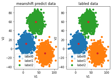
y_predict_ms = ms.predict(X)
print(pd.value_counts(y_predict_ms), pd.value_counts(y))

fig10 = plt.subplot(121)
label0 = plt.scatter(X.loc[:,'V1'][y_predict_ms==0],X.loc[:,'V2'][y_predict_ms==0])
label1 = plt.scatter(X.loc[:,'V1'][y_predict_ms==1],X.loc[:,'V2'][y_predict_ms==1])
label2 = plt.scatter(X.loc[:,'V1'][y_predict_ms==2],X.loc[:,'V2'][y_predict_ms==2])

plt.title("meanshift predict data")
plt.xlabel('V1')
plt.ylabel('V2')
plt.legend((label0,label1,label2),('label0','label1','label2'))
plt.scatter(centers[:,0],centers[:,1])

fig11 = plt.subplot(122)
label0 = plt.scatter(X.loc[:,'V1'][y==0],X.loc[:,'V2'][y==0])
label1 = plt.scatter(X.loc[:,'V1'][y==1],X.loc[:,'V2'][y==1])
label2 = plt.scatter(X.loc[:,'V1'][y==2],X.loc[:,'V2'][y==2])

plt.title("labled data")
plt.xlabel('V1')
plt.ylabel('V2')
plt.legend((label0,label1,label2),('label0','label1','label2'))
plt.scatter(centers[:,0],centers[:,1])
plt.show()

#矫正结果
y_corrected_ms = []
for i in y_predict_ms:
    if i==0:
        y_corrected_ms.append(2)
    elif i==1:
        y_corrected_ms.append(1)
    else:
        y_corrected_ms.append(0)
print(pd.value_counts(y_corrected_ms),pd.value_counts(y))

# convert the results to numpy array
y_corrected_ms = np.array(y_corrected_ms)
print(type(y_corrected_ms))

fig12 = plt.subplot(121)
label0 = plt.scatter(X.loc[:,'V1'][y_corrected_ms==0],X.loc[:,'V2'][y_corrected_ms==0])
label1 = plt.scatter(X.loc[:,'V1'][y_corrected_ms==1],X.loc[:,'V2'][y_corrected_ms==1])
label2 = plt.scatter(X.loc[:,'V1'][y_corrected_ms==2],X.loc[:,'V2'][y_corrected_ms==2])

plt.title("meanshift predict data")
plt.xlabel('V1')
plt.ylabel('V2')
plt.legend((label0,label1,label2),('label0','label1','label2'))
plt.scatter(centers[:,0],centers[:,1])

fig13 = plt.subplot(122)
label0 = plt.scatter(X.loc[:,'V1'][y==0],X.loc[:,'V2'][y==0])
label1 = plt.scatter(X.loc[:,'V1'][y==1],X.loc[:,'V2'][y==1])
label2 = plt.scatter(X.loc[:,'V1'][y==2],X.loc[:,'V2'][y==2])

plt.title("labled data")
plt.xlabel('V1')
plt.ylabel('V2')
plt.legend((label0,label1,label2),('label0','label1','label2'))
plt.scatter(centers[:,0],centers[:,1])
plt.show()

image