吴裕雄--天生自然 R语言开发学习：基础知识

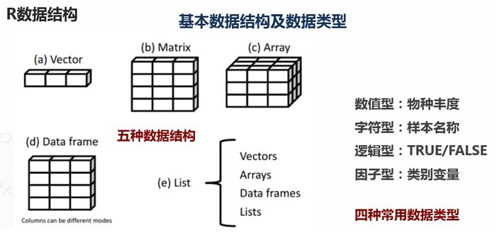
1.基础数据结构
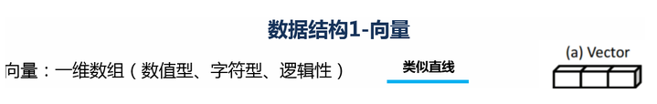
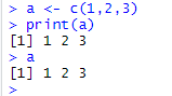
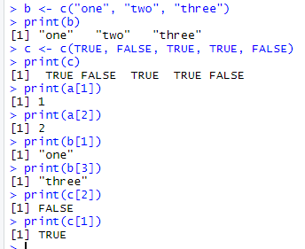
1.1 向量

# 创建向量a
a <- c(1,2,3)
print(a)

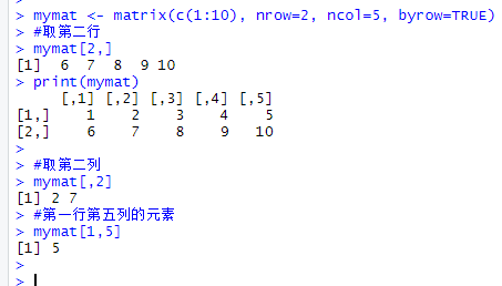
1.2 矩阵
#创建矩阵
mymat <- matrix(c(1:10), nrow=2, ncol=5, byrow=TRUE)
#取第二行
mymat[2,]
#取第二列
mymat[,2]
#第一行第五列的元素
mymat[1,5]

1.3 数组
#创建数组
myarr <- array(c(1:12),dim=c(2,3,2))
print(myarr)
#取矩阵或数组的维度
dim(myarr)
#取第一个矩阵的第一行第二列
myarr[1,2,1]

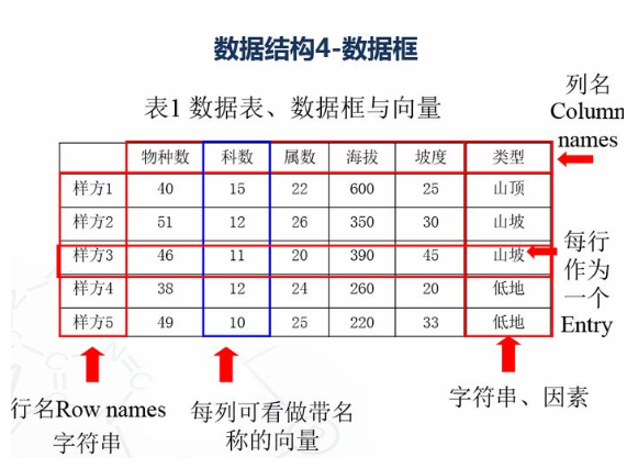
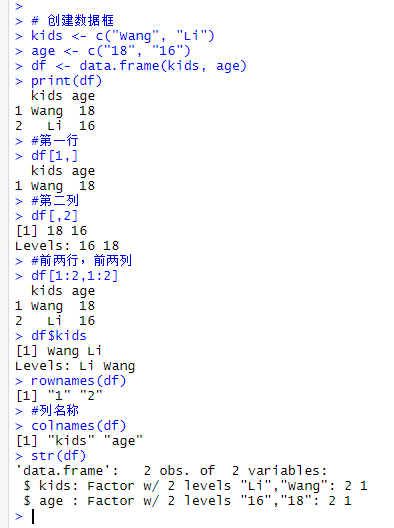
1.4 数据框
# 创建数据框
kids <- c("Wang", "Li")
age <- c("", "")
df <- data.frame(kids, age)
print(df)
#第一行
df[1,]
#第二列
df[,2]
#前两行，前两列
df[1:2,1:2]
#根据列名称
df$kids
#行名称
rownames(df)
#列名称
colnames(df)

str(df)

1.4.1 因子变量
变量：类别变量，数值变量
类别数据对于分组数据研究非常有用。（男女，高中低）
R中的因子变量类似于类别数据。

1.5 列表
列表以一种简单的方式组织和调用不相干的信息，R函数的许多运行结果都是以列表的形式返回

#创建列表
lis <- list(name='fred',wife='mary',no.children=3,child.ages=c(4,7,9))
print(lis)
#列表组件名
lis$name
#列表位置访问
lis[[1]] 

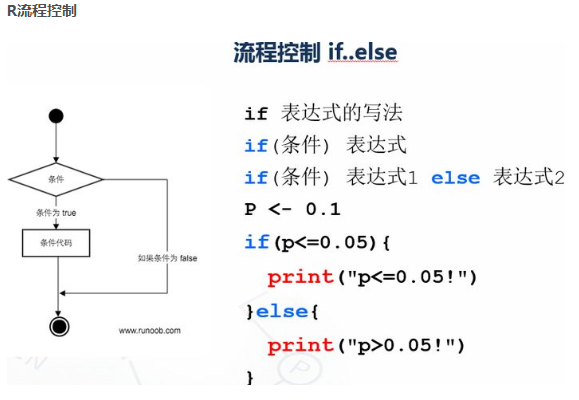
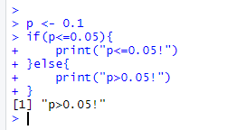
p <- 0.1
if(p<=0.05){
print("p<=0.05!")
}else{
print("p>0.05!")
}

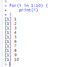
for(i in 1:10) {
print(i)
}

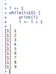
i <- 1
while(i<10) {
print(i)
i <- i + 1
  }

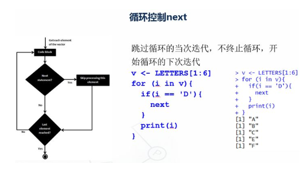
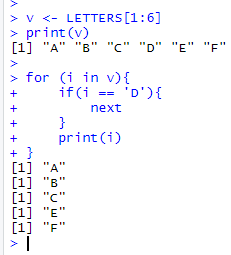
v <- LETTERS[1:6]
print(v)
for (i in v){
    if(i == 'D'){
        next
  }
  print(i)
}

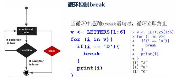
v <- LETTERS[1:6]
for (i in v){
    if(i == 'D'){
        break
  }
  print(i)
}

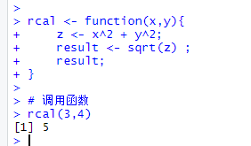
2.5 R函数
函数是组织好的，可重复使用的，用来实现单一，或相关联功能的代码段
rcal <- function(x,y){
  z <- x^2 + y^2;
  result <- sqrt(z) ;
  result;
}

# 调用函数
rcal(3,4)

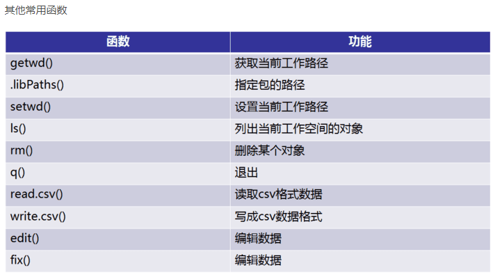
3. 读写数据
#数据读入
getwd()
setwd('C:/Users/Administrator/Desktop/file')
dir()
top <- read.table("otu_table.p10.relative.tran.xls",header=T,row.names=1,sep='\t',stringsAsFactors = F)
top10 <- t(top)
#数据写出logtop10<-log(top10+0.000001)
head(top10, n=2)
write.csv(logtop10,file="logtop10.csv", quote=FALSE,  row.names = TRUE)
write.table(logtop10,file="logtop10.xls",sep="\t", quote=FALSE, row.names = TRUE, col.names = TRUE)

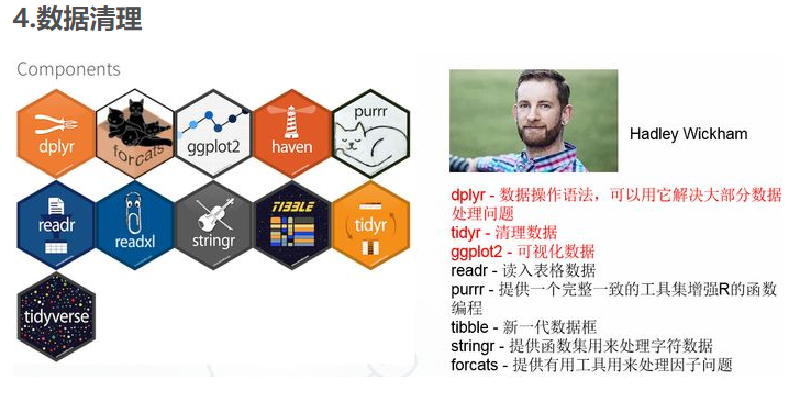
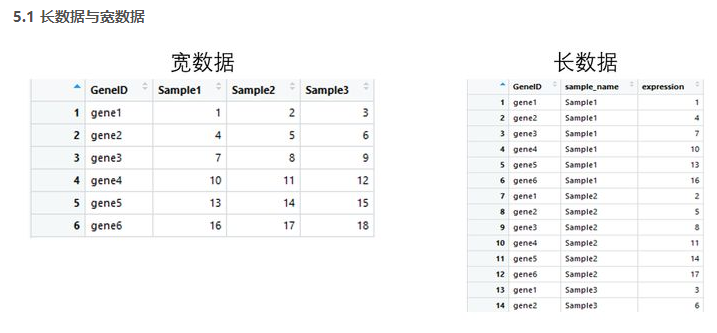
4.1 tidyr包
tidyr包的四个函数
宽数据转为长数据：gather()
长数据转为宽数据：spread()
多列合并为一列： unite()
将一列分离为多列：separate()

library(tidyr)
gene_exp <- read.table('geneExp.csv',header = T,sep=',',stringsAsFactors = F)
head(gene_exp)
#gather 宽数据转为长数据
gene_exp_tidy <- gather(data = gene_exp, key = "sample_name", value = "expression", -GeneID)
head(gene_exp_tidy)
#spread 长数据转为宽数据
gene_exp_tidy2<-spread(data = gene_exp_tidy, key = "sample_name", value = "expression")
head(gene_exp_tidy2)

4.2 dplyr包
dplyr包五个函数用法：
筛选: filter
排列: arrange()
选择: select()
变形: mutate()
汇总: summarise()
分组: group_by()

library(tidyr)
library(dplyr)
gene_exp <- read.table("geneExp.csv",header=T,sep=",",stringsAsFactors = F)
gene_exp_tidy <- gather(data = gene_exp, key = "sample_name", value = "expression", -GeneID)
#arrange 数据排列
gene_exp_GeneID <- arrange(gene_exp_tidy, GeneID)
#降序加
deschead(gene_exp_GeneID )
#filter 数据按条件筛选
gene_exp_fiter <- filter(gene_exp_GeneID ,expression>10)
head(gene_exp_fiter)
#select 选择对应的列
gene_exp_select <- select(gene_exp_fiter ,sample_name,expression)
head(gene_exp_select)

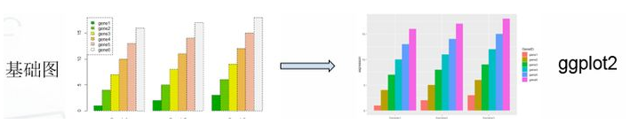
library(tidyr)
library(ggplot2)
#基础绘图
#宽数据file
file <- read.table("geneExp.csv",header=T,sep=",",stringsAsFactors = F,row.names = 1)
barplot(as.matrix(file),names.arg = colnames(file), beside =T ,col=terrain.colors(6))
legend("topleft",legend = rownames(file),fill = terrain.colors(6))
#ggplot2绘图
gene_exp <- read.table("geneExp.csv",header=T,sep=",",stringsAsFactors = F)
gene_exp_tidy <- gather(data = gene_exp, key = "sample_name", value = "expression", -GeneID)
#长数据head(gene_exp_tidy)
ggplot(gene_exp_tidy,aes(x=sample_name,y=expression,fill=GeneID)) + geom_bar(stat='identity',position='dodge')

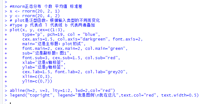
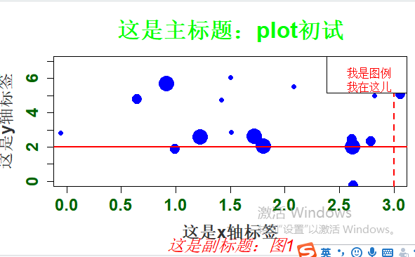
#Rnorm正态分布 个数 平均值 标准差
x <- rnorm(20, 2, 1)
y <- rnorm(20, 4, 2)
# plot是泛型函数，根据输入类型的不同而变化
#Type p 代表点 l 代表线 b 代表两者叠加
plot(x, y, cex=c(1:3),
type="p", pch=19, col = "blue",
cex.axis=1.5, col.axis="darkgreen", font.axis=2,
main="这是主标题：plot初试",
font.main=2, cex.main=2, col.main="green",
sub="这是副标题：图1",
font.sub=3, cex.sub=1.5, col.sub="red",
xlab="这是x轴标签",
ylab="这是y轴标签",
cex.lab=1.5, font.lab=2, col.lab="grey20",
xlim=c(0,3),
ylim=c(0,7))

abline(h=2, v=3, lty=1:2, lwd=2,col="red")
legend("topright", legend="我是图例\n我在这儿",text.col="red", text.width=0.5)
 

图形参数：
符号和线条：pch、cex、lty、lwd
颜色：col、col.axis、col.lab、col.main、col.sub、fg、bg
文本属性：cex、cex.axis、cex.lab、cex.main、cex.sub、font、font.axis、font.lab、font.main、font.sub

文本添加、坐标轴的自定义和图例
title()、main、sub、xlab、ylab、text()
axis()、abline()
legend()

多图绘制时候，可使用par()设置默认的图形参数
par(lwd=2, cex=1.5)

图形参数设置：
par(optionname=value,…)
par(pin=c(width,height)) 图形尺寸
par(mfrow=c(nr,nc)) 图形组合，一页多图
layout(mat) 图形组合，一页多图
par(mar=c(bottom,left,top,right)) 边界尺寸
par(fig=c(x1,x2,y1,y2),new=TURE) 多图叠加或排布成一幅图

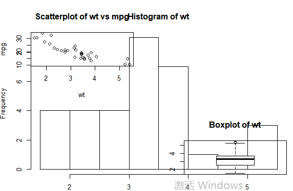
#图形组合：
attach(mtcars)
#复制当前图形参数设置
opar <- par(no.readonly=TRUE)
#设置图形参数
par(mfrow=c(2,2))
layout(matrix(c(1,2,2,3),2,2,byrow=TRUE))
plot(wt,mpg,main="Scatterplot of wt vs mpg")
hist(wt,main="Histogram of wt")
boxplot(wt,main="Boxplot of wt")
#返回原始图形参数detach(mtcars)
par(opar) 

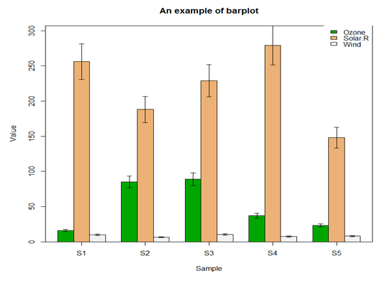
5.3 柱形图

file <- read.table("barData.csv",header=T,row.names=1,sep=",",stringsAsFactors = F)
#转化为矩阵
dataxx <- as.matrix(file)
#抽取颜色
cols <- terrain.colors(3)
#误差线函数
plot.error <- function(x, y, sd, len = 1, col = "black") {
    len <- len * 0.05
    arrows(x0 = x, y0 = y, x1 = x, y1 = y - sd, col = col, angle = 90, length = len)
    arrows(x0 = x, y0 = y, x1 = x, y1 = y + sd, col = col, angle = 90, length = len)
}
x <- barplot(dataxx, offset = 0, ylim=c(0, max(dataxx) * 1.1),axis.lty = 1, names.arg = colnames(dataxx), col = cols, beside = TRUE)
box()
legend("topright", legend = rownames(dataxx), fill = cols, box.col = "transparent")
title(main = "An example of barplot", xlab = "Sample", ylab = "Value")
sd <- dataxx * 0.1
for (i in 1:3) {
  plot.error(x[i, ], dataxx[i, ], sd = sd[i, ])
}

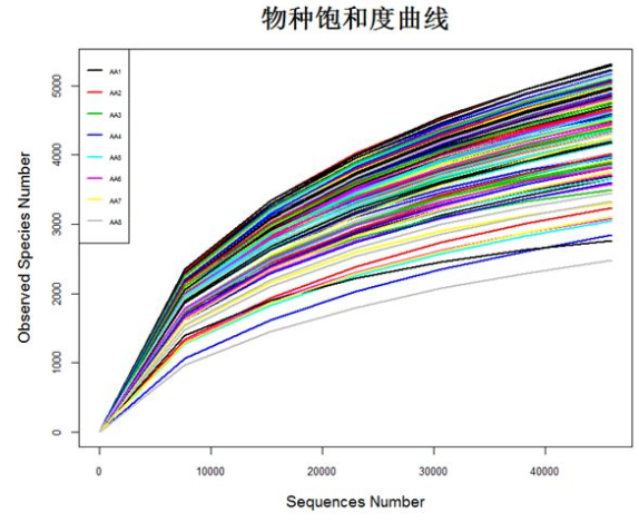
5.4 二元图

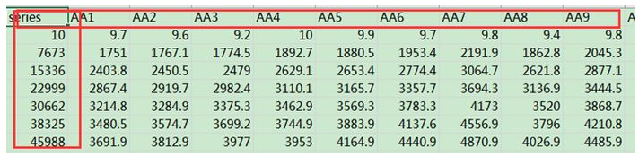
matdata <- read.table("plot_observed_species.xls", header=T)
#查看数据属性和结构
tbl_df(matdata)
y<-matdata[,2:145]
attach(matdata)
matplot(series,y,
        ylab="Observed Species Number",xlab="Sequences Number",
        lty=1,lwd=2,type="l",col=1:145,cex.lab=1.2,cex.axis=0.8)
legend("topleft",lty=1, lwd=2, legend=names(y)[1:8], cex=0.5,col=1:145)
detach(matdata)

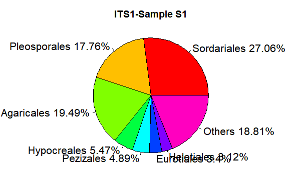
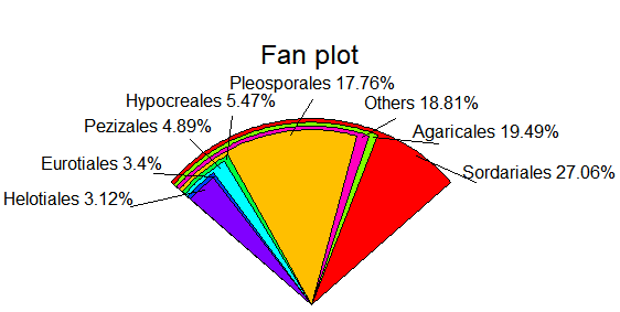
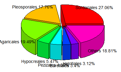
5.5 饼状图

relative <- c(0.270617,0.177584,0.194911,0.054685,0.048903,0.033961, 0.031195,0.188143)
taxon <- c("Sordariales","Pleosporales","Agaricales","Hypocreales","Pezizales","Eurotiales","Helotiales","Others")
ratio <- round(relative*100,2)
ratio <- paste(ratio,"%",sep="")
label <- paste(taxon,ratio,sep=" ")
pie(relative,labels=label, main="ITS1-Sample S1",radius=1,col=rainbow(length(label)),cex=1.3)

library(plotrix)
fan.plot(relative,labels=label,main="Fan plot")

pie3D(relative,labels=label, height=0.2, theta=pi/4, explode=0.1, col=rainbow(length(label)),border="black",font=2,radius=1,labelcex=0.9)

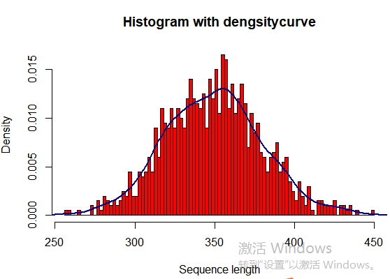
5.6 直方图

seqlength <- rnorm(1000, 350, 30)

hist(seqlength,breaks=100,col="red",
freq=FALSE,
main="Histogram with dengsitycurve",
ylab="Density",
xlab="Sequence length")
lines(density(seqlength),col="blue4",lwd=2)

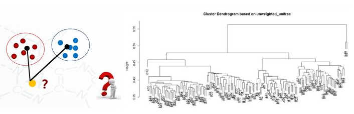
5.7 聚类图

clu <- read.table("unweighted_unifrac_dm.txt", header=T, row.names=1, sep="\t")
head(clu)
dis <- as.dist(clu)
h <- hclust(dis, method="average")
plot(h, hang = 0.1, axes = T, frame.plot = F, main="Cluster Dendrogram based on unweighted_unifrac", sub="UPGMA")

#保存图片代码
pdf(file="file.pdf", width=7, height=10)
png(file="file.png",width=480,height=480)
jpeg(file="file.png",width=480,height=480)
tiff(file="file.png",width=480,height=480)

dev.off()