A Statistical View of Deep Learning (IV): Recurrent Nets and Dynamical Systems

Recurrent neural networks (RNNs) are now established as one of the key tools in the machine learning toolbox for handling large-scale sequence data. The ability to specify highly powerful models, advances in stochastic gradient descent, the availability of large volumes of data, and large-scale computing infrastructure, now allows us to apply RNNs in the most creative ways. From handwriting generation, image captioning, language translation and voice recognition, RNNs now routinely find themselves as part of large-scale consumer products.

On a first encounter, there is a mystery surrounding these models. We refer to them under many different names: as recurrent networks in deep learning, as state space models in probabilistic modelling, as dynamical systems in signal processing, and as autonomousand non-autonomous systems in mathematics. Since they attempt to solve the same problem, these descriptions are inherently bound together and many lessons can be exchanged between them: in particular, lessons on large-scale training and deployment for big data problems from deep learning, and even more powerful sequential models such aschangepoint, factorial or switching state-space models. This post is an initial exploration of these connections.

Equivalent models: recurrent networks and state-space models.

Recurrent Neural Networks

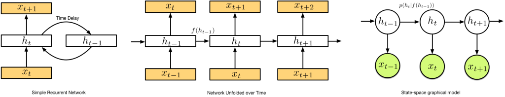
Recurrent networks [1] take a functional viewpoint to sequence modelling. They describe sequence data using a function built using recursive components that use feedback from hidden units at time points in the past to inform computations of the sequence at the present. What we obtain is a neural network where activations of one of the hidden layers feeds back into the network along with the input (see figures). Such a recursive description is unbounded and to practically use such a model, we unfold the network in time and explicitly represent a fixed number of recurrent connections. This transforms the model into a feedforward network for which our familiar techniques can be applied.

If we consider an observed sequence x, we can describe a loss function for RNNs unfolded for T steps as:

Feedback:ht=fθ(h<t,xt−1)

Loss:J(θ)=∑t=1Td(xt,ht)

The model and corresponding loss function is that of a feedforward network, with d(.) an appropriate distance function for the data being predicted, such as the squared loss. The difference from standard feedforward networks is that the parameters θ of the recursive function f are the same for all time points, i.e. they are shared across the model. We can perform parameter estimation by averaging over a mini-batch of sequences and using stochastic gradient descent with application of the backpropagation algorithm. For recurrent networks, this combination of unfolding in time and backpropagation is referred to as backpropagation through time (BPTT) [2].

Since we have simplified our task by always considering the learning algorithm as the application of SGD and backprop, we are free to focus our energy on creative specifications of the recursive function. The simplest and common recurrent networks use feedback from one past hidden layer— earlier examples include the Elman or Jordan networks. But the true workhorse of current recurrent deep learning is the Long Short-Term Memory (LSTM) network [3]. The transition function in an LSTM produces two hidden vectors: a hidden layer h, and a memory cell c, and applies the function f composed of soft-gating using sigmoid functions σ(.) and a number of weights and biases (e.g., A, B,a, b):

Input:it=σ(Axt+Bht−1+Dct−1+a)

Forget:ft=σ(Ext+Fht−1+Gct−1+b)

Cell:ct=ftct−1+ittanh(Hxt+Ght−1+d)

Output:ot=σ(Kxt+Lht−1+Mct+e)

Hidden:ht=ottanh(ct)

Probabilistic dynamical systems

We can also view the recurrent network construction above using a probabilistic framework (relying on reasoning used in part I of this series). Instead of viewing the recurrent network as a recursive function followed by unfolding for T time steps, we can directly model a sequence of length T with latent (or hidden) dynamics and specify aprobabilistic graphical model. Both the latent states h and the observed data x are assumed to be probabilistic. The transition probability is the same for all time, so this is equivalent to assuming the parameters of the transition function are shared. We could refer to these models as stochastic recurrent networks; the established convention is to refer to them as dynamical systems or state-space models.

In probabilistic modelling, the core quantity of interest is the probability of the observed sequence x, computed as follows:

p(x1,…xT)=∏t∫p(xt,ht)dht

p(xt,ht)=p(xt|ht)p(ht|ht−1)

Using maximum likelihood estimation, we can obtain a loss function based on the log of this marginal likelihood. Since for recurrent networks the transition dynamics is assumed to be deterministic, we can easily recover the RNN loss function:

Det. Dynamics:pθ(ht|ht−1)=δ(ht=fθ(ht−1,xt−1))

Loss:J(θ)=∑tlog∫p(ht|ht−1)p(xt|ht)dht

⟹J(θ)=∑tlogp(xt|fθ(ht−1,xt−1))

which recovers the original loss function with the distance function given by the log of the chosen likelihood function. It is no surprise that the RNN loss corresponds to maximum likelihood estimation with deterministic dynamics.

As machine learners we never really trust our data, so in some cases we will wish to consider noisy observations and stochastic transitions. We may also wish to explore estimation beyond maximum likelihood. A great deal of power is obtained by considering stochastic transitions that transform recurrent networks into probabilistic generative temporal models [4][5] — models that account for missing data, allow for denoising and built-in regularisation, and that model the sequence density. We gain new avenues for creativity in our transitions: we can now consider states that jump and random times between different operational modes, that might reset to a base state, or that interact with multiple sequences simultaneously.

But when the hidden states h are random, we are faced with the problem of inference. For certain assumptions such as discrete or Gaussian transitions, algorithms for hidden Markov models and Kalman filters, respectively, demonstrate ways in which this can be done. More recent approaches use variational inference or particle MCMC [4]. In general, efficient inference for large-scale state-space models remains an active research area.

Prediction, Filtering and Smoothing

Dynamical systems are often described to make three different types of inference problems explicit: prediction, filtering and smoothing [5].

Prediction (inferring the future) is the first use of most machine learning models. Having seen training data we are asked to forecast the behaviour of the sequence at some point k time-steps in the future. Here, we compute the predictive distribution of the hidden state, since knowing this allows us to predict or generate what would be observed: p(ht+k|y1,…t)
Filtering (inferring the present) is the task of computing the marginal distribution of the hidden state given only the past states and observations. p(ht|y1,…,t)
Smoothing (inferring the past) is the task of computing the marginal distribution of the hidden state given knowledge of the past and future observations. p(ht|y1,…,T),t<T.

These operations neatly separate the different types of computations that must be performed to correctly reason about the sequence with random hidden states. For RNNs, due to their deterministic nature, computing predictive distributions and filtering are realised by the feedforward operations in the unfolded network. Smoothing is an operation that does not have a counterpart, but architectures such as bi-directional recurrent nets attempt to fill this role.

Summary

Recurrent networks and state space models attempt to solve the same problem: how to best reason from sequential data. As we continue research in this area, it is the intersection of deterministic and probabilistic approaches that will allow us to further exploit the power of these temporal models. Recurrent networks have been shown to be powerful, scalable, and applicable to an incredibly diverse set of problems. They also have much to teach in terms of initialisation, stability issues, gradient management and the implementation of large-scale temporal models. Probabilistic approaches have much to offer in terms of better regularisation, different types of sequences we can model, and the wide range of probabilistic queries we can make with models of sequence data. There is much more that can be said, but these initial connections make clear the way forward.

Some References

[1]	Yoshua Bengio, Ian Goodfellow, Aaron Courville, Deep Learning, , 2015
[2]	Paul J Werbos, Backpropagation through time: what it does and how to do it, Proceedings of the IEEE, 1990
[3]	Felix. Gers, Long short-term memory in recurrent neural networks, , 2011
[4]	David Barber, A Taylan Cemgil, Silvia Chiappa, Bayesian time series models, , 2011
[5]	Simo S\"arkk\"a, Bayesian filtering and smoothing, , 2013