《DSP using MATLAB》 Problem 3.19

先求模拟信号经过采样后，对应的数字角频率：

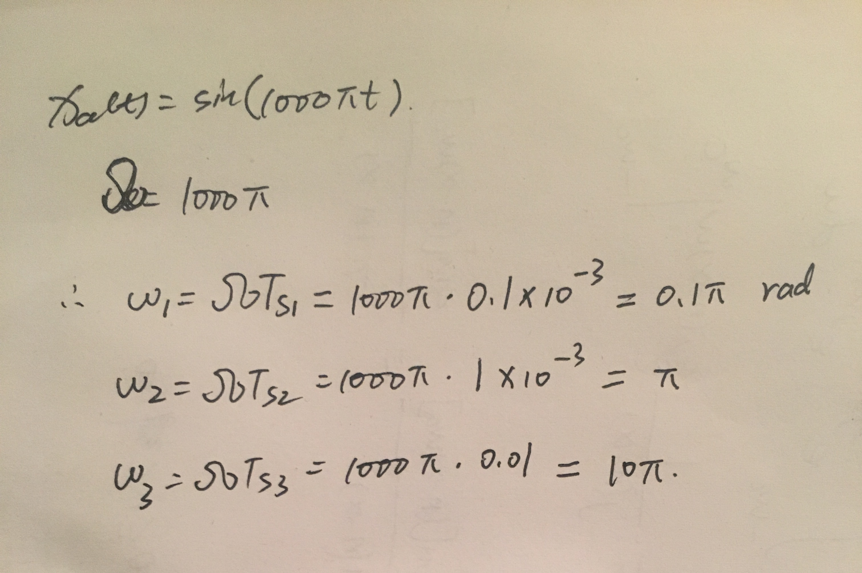
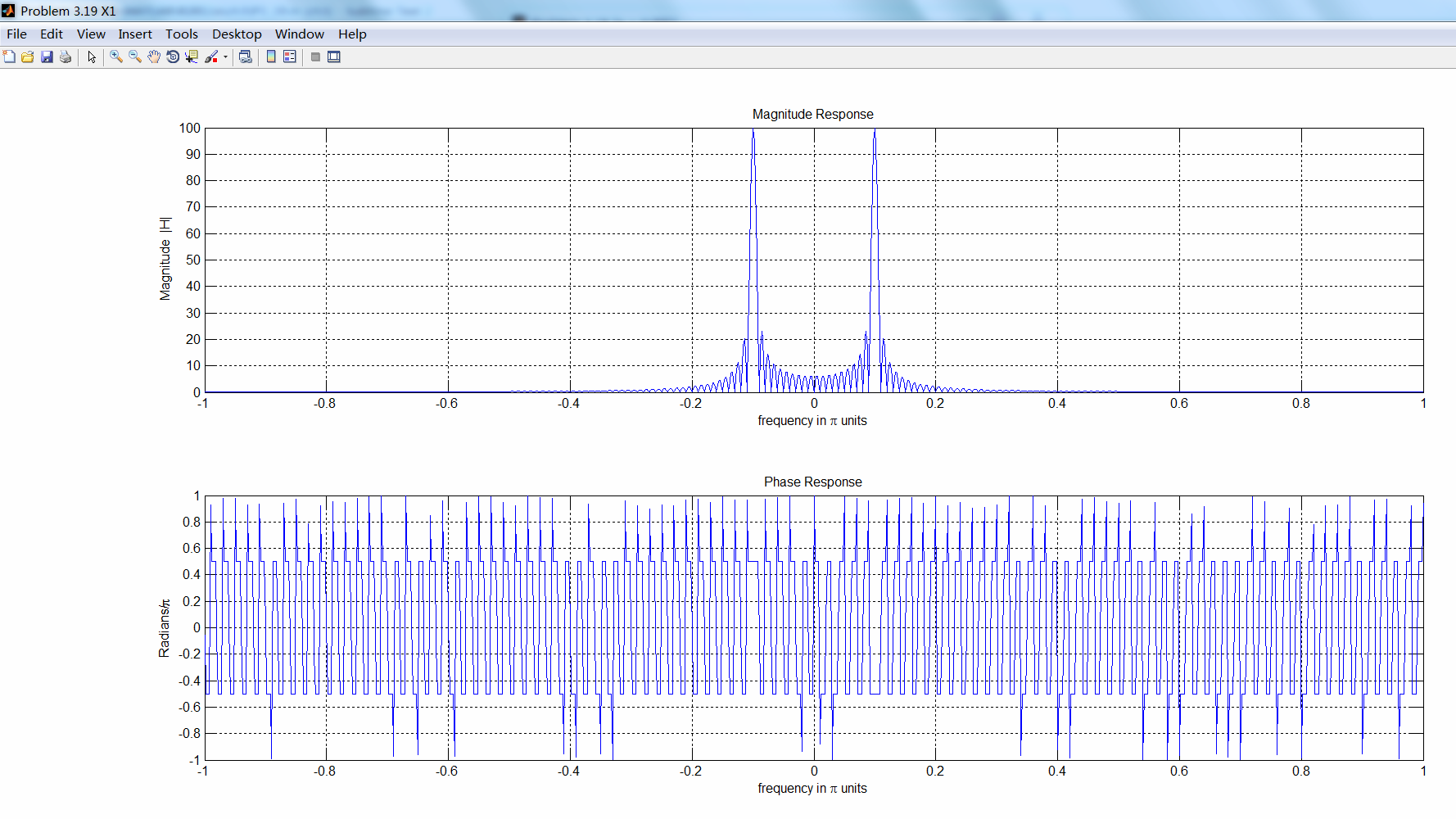
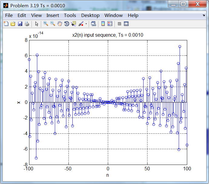
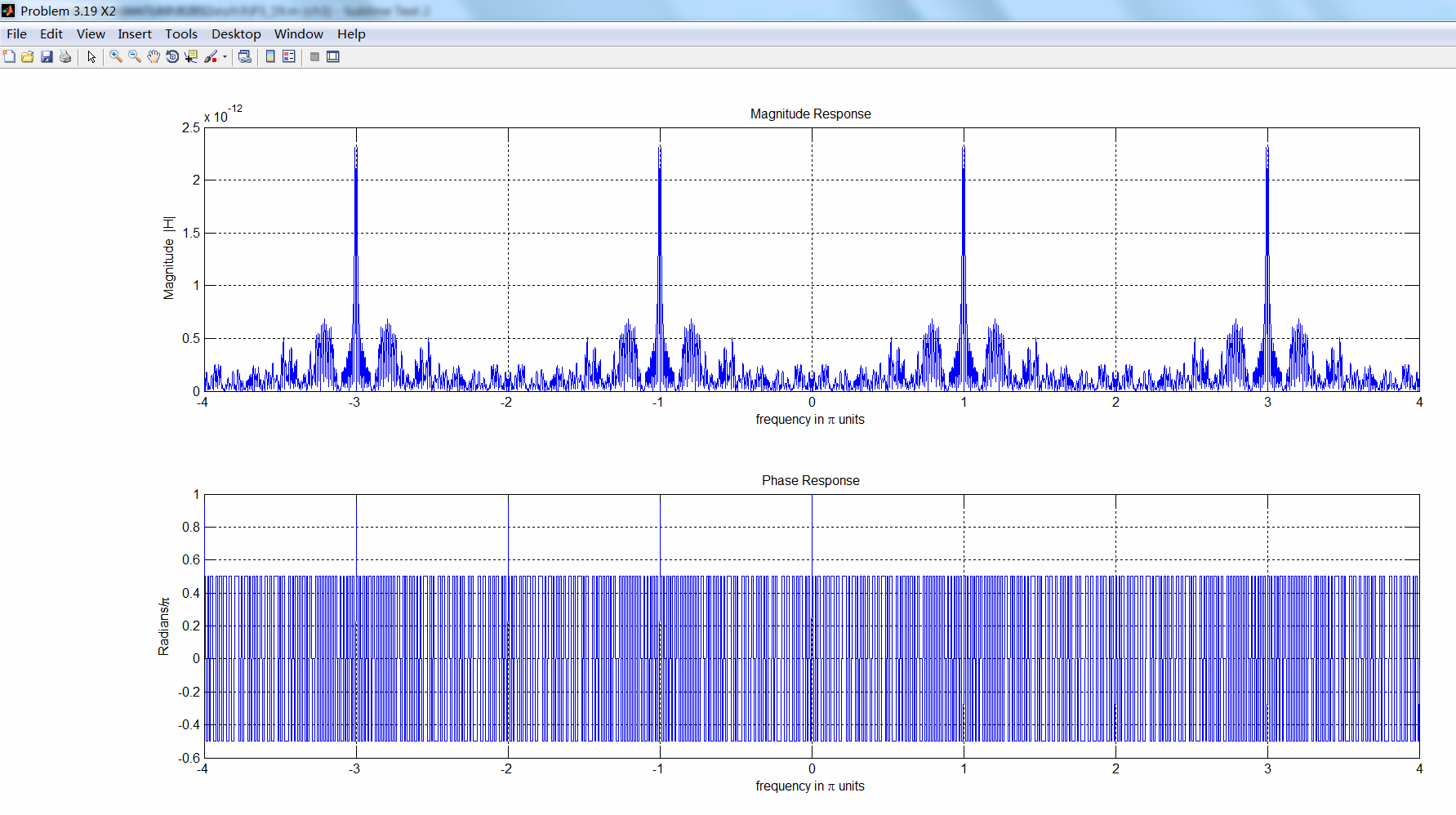
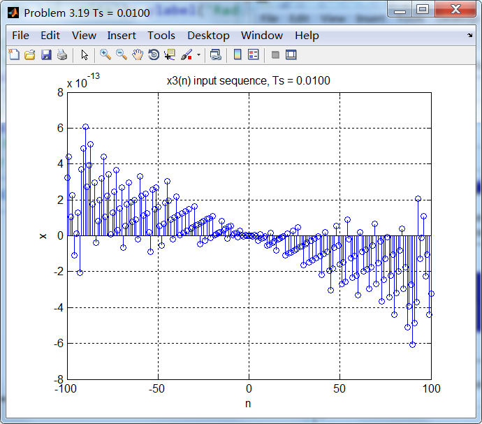
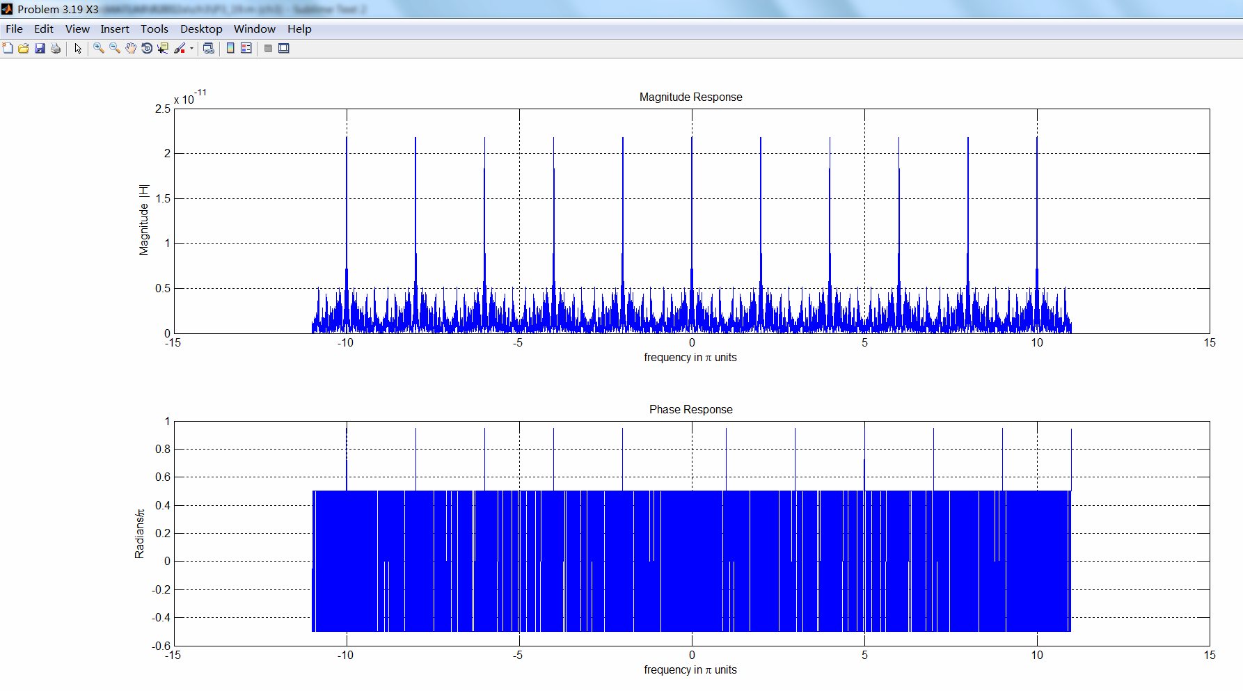
明显看出，第3种采样出现假频了。DTFT是以2π为周期的，所以假频出现在10π-2kπ=0处。

代码：

%% ------------------------------------------------------------------------
%%            Output Info about this m-file
fprintf('\n***********************************************************\n');
fprintf('        <DSP using MATLAB> Problem 3.19 \n\n');

banner();
%% ------------------------------------------------------------------------

%% -------------------------------------------------------------------
%%                     xa(t)=sin(1000pit)
%% -------------------------------------------------------------------
Ts = 0.0001;         % second unit
n1 = [-100:100];

x1 = sin(1000*pi*n1*Ts);

figure('NumberTitle', 'off', 'Name', sprintf('Problem 3.19 Ts = %.4f', Ts));
set(gcf,'Color','white');
%subplot(2,1,1);
stem(n1, x1);
xlabel('n'); ylabel('x');
title(sprintf('x1(n) input sequence, Ts = %.4f', Ts)); grid on;

M = 500;
[X1, w] = dtft1(x1, n1, M);

magX1  = abs(X1);  angX1  = angle(X1);  realX1  = real(X1);  imagX1  = imag(X1);

%% --------------------------------------------------------------------
%%              START X(w)'s  mag ang real imag
%% --------------------------------------------------------------------
figure('NumberTitle', 'off', 'Name', 'Problem 3.19 X1');
set(gcf,'Color','white');
subplot(2,1,1); plot(w/pi,magX1); grid on;  %axis([-1,1,0,1.05]);
title('Magnitude Response');
xlabel('frequency in \pi units'); ylabel('Magnitude  |H|');
subplot(2,1,2); plot(w/pi, angX1/pi); grid on;  %axis([-1,1,-1.05,1.05]);
title('Phase Response');
xlabel('frequency in \pi units'); ylabel('Radians/\pi');

figure('NumberTitle', 'off', 'Name', 'Problem 3.19 X1');
set(gcf,'Color','white');
subplot(2,1,1); plot(w/pi, realX1); grid on;
title('Real Part');
xlabel('frequency in \pi units'); ylabel('Real');
subplot(2,1,2); plot(w/pi, imagX1); grid on;
title('Imaginary Part');
xlabel('frequency in \pi units'); ylabel('Imaginary');
%% -------------------------------------------------------------------
%%             END X's  mag ang real imag
%% -------------------------------------------------------------------

% ----------------------------------------------------------
%                Ts=0.001s
% ----------------------------------------------------------
Ts = 0.001;         % second unit
n2 = [-100:100];

x2 = sin(1000*pi*n2*Ts);

figure('NumberTitle', 'off', 'Name', sprintf('Problem 3.19 Ts = %.4f', Ts));
set(gcf,'Color','white');
%subplot(2,1,1);
stem(n2, x2);
xlabel('n'); ylabel('x');
title(sprintf('x2(n) input sequence, Ts = %.4f', Ts)); grid on;

M = 500;
[X2, w] = dtft1(x2, n2, M);

magX2  = abs(X2);  angX2  = angle(X2);  realX2  = real(X2);  imagX2  = imag(X2);

%% --------------------------------------------------------------------
%%              START X(w)'s  mag ang real imag
%% --------------------------------------------------------------------
figure('NumberTitle', 'off', 'Name', 'Problem 3.19 X2');
set(gcf,'Color','white');
subplot(2,1,1); plot(w/pi,magX2); grid on;  %axis([-1,1,0,1.05]);
title('Magnitude Response');
xlabel('frequency in \pi units'); ylabel('Magnitude  |H|');
subplot(2,1,2); plot(w/pi, angX2/pi); grid on;  %axis([-1,1,-1.05,1.05]);
title('Phase Response');
xlabel('frequency in \pi units'); ylabel('Radians/\pi');

figure('NumberTitle', 'off', 'Name', 'Problem 3.19 X2');
set(gcf,'Color','white');
subplot(2,1,1); plot(w/pi, realX2); grid on;
title('Real Part');
xlabel('frequency in \pi units'); ylabel('Real');
subplot(2,1,2); plot(w/pi, imagX2); grid on;
title('Imaginary Part');
xlabel('frequency in \pi units'); ylabel('Imaginary');
%% -------------------------------------------------------------------
%%             END X's  mag ang real imag
%% -------------------------------------------------------------------

% ----------------------------------------------------------
%                Ts=0.01s
% ----------------------------------------------------------
Ts = 0.01;         % second unit
n3 = [-100:100];

x3 = sin(1000*pi*n3*Ts);

figure('NumberTitle', 'off', 'Name', sprintf('Problem 3.19 Ts = %.4f', Ts));
set(gcf,'Color','white');
%subplot(2,1,1);
stem(n3, x3);
xlabel('n'); ylabel('x');
title(sprintf('x3(n) input sequence, Ts = %.4f', Ts)); grid on;

M = 500;
[X3, w] = dtft1(x3, n3, M);

magX3  = abs(X3);  angX3  = angle(X3);  realX3  = real(X3);  imagX3  = imag(X3);

%% --------------------------------------------------------------------
%%              START X(w)'s  mag ang real imag
%% --------------------------------------------------------------------
figure('NumberTitle', 'off', 'Name', 'Problem 3.19 X3');
set(gcf,'Color','white');
subplot(2,1,1); plot(w/pi,magX3); grid on;  %axis([-1,1,0,1.05]);
title('Magnitude Response');
xlabel('frequency in \pi units'); ylabel('Magnitude  |H|');
subplot(2,1,2); plot(w/pi, angX3/pi); grid on;  %axis([-1,1,-1.05,1.05]);
title('Phase Response');
xlabel('frequency in \pi units'); ylabel('Radians/\pi');

figure('NumberTitle', 'off', 'Name', 'Problem 3.19 X3');
set(gcf,'Color','white');
subplot(2,1,1); plot(w/pi, realX3); grid on;
title('Real Part');
xlabel('frequency in \pi units'); ylabel('Real');
subplot(2,1,2); plot(w/pi, imagX3); grid on;
title('Imaginary Part');
xlabel('frequency in \pi units'); ylabel('Imaginary');
%% -------------------------------------------------------------------
%%             END X's  mag ang real imag
%% -------------------------------------------------------------------

　　运行结果：

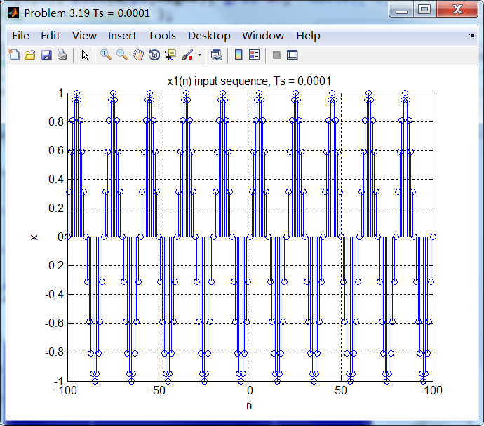
采样后的序列及其谱。