《DSP using MATLAB》Problem 5.19

代码：

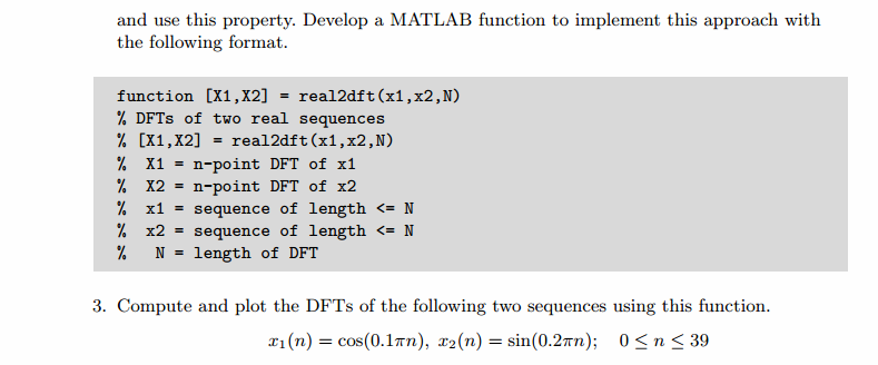
function [X1k, X2k] = real2dft(x1, x2, N)
    %% ---------------------------------------------------------------------
	%%    DFT of two Real-Valued N-Point sequence x1(n) and x2(n)
	%% ---------------------------------------------------------------------
	%% [X1, X2] = real2dft(x1, x2, N)
	%%      X1k = n-point DFT of x1
	%%      X2k = n-point DFT of x2
	%%       x1 = sequence of length <= N
	%%       x2 = sequence of length <= N
	%%       N  = length of DFT

	% ----------------------------------------
	%    if length of x1 and x2 < N,
	%       then padding zeros
	% ----------------------------------------
	if ( length(x1) < N)
		x1 = [x1 zeros(1, N-length(x1))];
    end

	if ( length(x2) < N)
		x2 = [x2 zeros(1, N-length(x2))];
    end

	x = x1 + j * x2;

	N = length(x); k = 0:(N-1); 

    Xk_DFT = dft(x, N);
    Xk_DFT_fold = Xk_DFT(mod_1(-k,N)+1);

    Xk_CCS = 0.5*(Xk_DFT + conj(Xk_DFT_fold));
    Xk_CCA = 0.5*(Xk_DFT - conj(Xk_DFT_fold));

	X1k = Xk_CCS;
	X2k = Xk_CCA;

　　

%% ++++++++++++++++++++++++++++++++++++++++++++++++++++++++++++++++++++++++++++++++++++++++
%%            Output Info about this m-file
fprintf('\n***********************************************************\n');
fprintf('        <DSP using MATLAB> Problem 5.19 \n\n');

banner();
%% ++++++++++++++++++++++++++++++++++++++++++++++++++++++++++++++++++++++++++++++++++++++++

% ---------------------------------------------------------------------------------
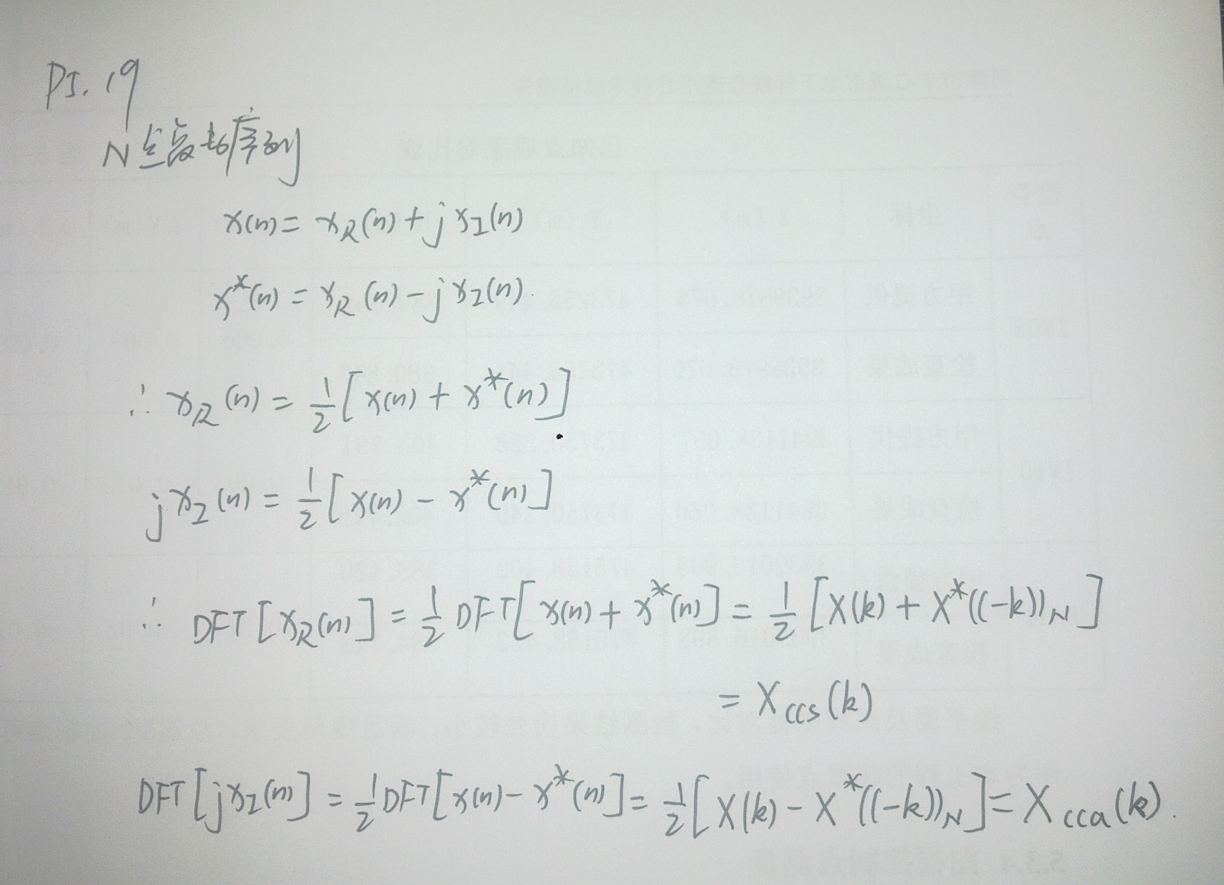
%          X(k) is N-point DFTs of N-point Complex-valued sequence x(n)
%               x(n) = xR(n) + j xI(n)
%            xR(n) and xI(n) are real and image parts of x(n);
%            DFT[xR]=Xccs(k)   DFT[j*xI]=Xcca(k)
%
%            Xccs = 0.5*[X(k)+ X*((-k))]      Xcca = 0.5*[X(k) - X*((-k))]
%
% ---------------------------------------------------------------------------------
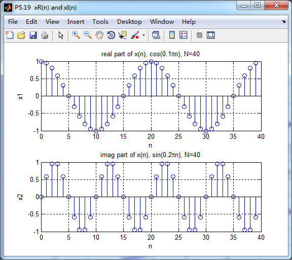
 n = [0:39];
x1 = cos(0.1*pi*n);                 % N=40 real-valued sequence
x2 = sin(0.2*pi*n);                 % N=40 real-valued sequence

x = x1 + j * x2;

N = length(x); k = 0:(N-1); 

    Xk_DFT = dft(x, N);
    Xk_DFT_fold = Xk_DFT(mod_1(-k,N)+1);

    magXk_DFT = abs( [ Xk_DFT ] );                                    % DFT magnitude
    angXk_DFT = angle( [Xk_DFT] )/pi;                                 % DFT angle
   realXk_DFT = real(Xk_DFT);
   imagXk_DFT = imag(Xk_DFT);

    magXk_DFT_fold = abs( [ Xk_DFT_fold ] );                                    % DFT magnitude
    angXk_DFT_fold = angle( [Xk_DFT_fold] )/pi;                                 % DFT angle
   realXk_DFT_fold = real(Xk_DFT_fold);
   imagXk_DFT_fold = imag(Xk_DFT_fold);

% --------------------------------------------------------
%        Calculater one N-point DFT to get
%                two N-point DFT
% --------------------------------------------------------
[X1k_DFT, X2k_DFT] = real2dft(x1, x2, N);

    magX1k_DFT = abs( [ X1k_DFT ] );                                    % DFT magnitude
    angX1k_DFT = angle( [X1k_DFT] )/pi;                                 % DFT angle
   realX1k_DFT = real(X1k_DFT);
   imagX1k_DFT = imag(X1k_DFT);

    magX2k_DFT = abs( [ X2k_DFT ] );                                    % DFT magnitude
    angX2k_DFT = angle( [X2k_DFT] )/pi;                                 % DFT angle
   realX2k_DFT = real(X2k_DFT);
   imagX2k_DFT = imag(X2k_DFT);

% -------------------------------------------------------
%         Get DFT of xR and xI directorly
% -------------------------------------------------------
XRk_DFT = dft(x1, N);
XIk_DFT = dft(j*x2, N);

    magXRk_DFT = abs( [ XRk_DFT ] );                                    % DFT magnitude
    angXRk_DFT = angle( [XRk_DFT] )/pi;                                 % DFT angle
   realXRk_DFT = real(XRk_DFT);
   imagXRk_DFT = imag(XRk_DFT);

    magXIk_DFT = abs( [ XIk_DFT ] );                                    % DFT magnitude
    angXIk_DFT = angle( [XIk_DFT] )/pi;                                 % DFT angle
   realXIk_DFT = real(XIk_DFT);
   imagXIk_DFT = imag(XIk_DFT);

figure('NumberTitle', 'off', 'Name', 'P5.19  xR(n) and xI(n)')
set(gcf,'Color','white');
subplot(2,1,1); stem(n, x1);
xlabel('n'); ylabel('x1');
title('real part of x(n), cos(0.1\pin), N=40');  grid on;
subplot(2,1,2); stem(n, x2);
xlabel('n'); ylabel('x2');
title('imag part of x(n), sin(0.2\pin), N=40');  grid on;

figure('NumberTitle', 'off', 'Name', 'P5.19 X(k), DFT of x(n)')
set(gcf,'Color','white');
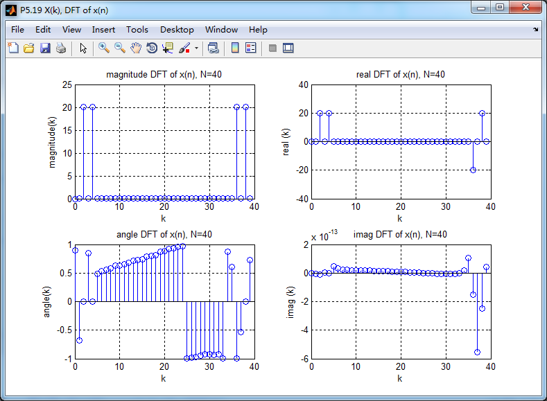
subplot(2,2,1); stem(k, magXk_DFT);
xlabel('k'); ylabel('magnitude(k)');
title('magnitude DFT of x(n), N=40');  grid on;
subplot(2,2,3); stem(k, angXk_DFT);
%axis([-N/2, N/2, -0.5, 50.5]);
xlabel('k'); ylabel('angle(k)');
title('angle DFT of x(n), N=40');  grid on;
subplot(2,2,2); stem(k, realXk_DFT);
xlabel('k'); ylabel('real (k)');
title('real DFT of x(n), N=40');  grid on;
subplot(2,2,4); stem(k, imagXk_DFT);
%axis([-N/2, N/2, -0.5, 50.5]);
xlabel('k'); ylabel('imag (k)');
title('imag DFT of x(n), N=40');  grid on;

figure('NumberTitle', 'off', 'Name', 'P5.19 X((-k))_N')
set(gcf,'Color','white');
subplot(2,2,1); stem(k, magXk_DFT_fold);
xlabel('k'); ylabel('magnitude(k)');
title('magnitude X((-k)), N=40');  grid on;
subplot(2,2,3); stem(k, angXk_DFT_fold);
%axis([-N/2, N/2, -0.5, 50.5]);
xlabel('k'); ylabel('angle(k)');
title('angle X((-k)), N=40');  grid on;
subplot(2,2,2); stem(k, realXk_DFT_fold);
xlabel('k'); ylabel('real (k)');
title('real X((-k)), N=40');  grid on;
subplot(2,2,4); stem(k, imagXk_DFT_fold);
%axis([-N/2, N/2, -0.5, 50.5]);
xlabel('k'); ylabel('imag (k)');
title('imag X((-k)), N=40');  grid on;

figure('NumberTitle', 'off', 'Name', 'P5.19 X1(k) by real2dft')
set(gcf,'Color','white');
subplot(2,2,1); stem(k, magX1k_DFT);
xlabel('k'); ylabel('magnitude(k)');
title('magnitude, N=40');  grid on;
subplot(2,2,3); stem(k, angX1k_DFT);
%axis([-N/2, N/2, -0.5, 50.5]);
xlabel('k'); ylabel('angle(k)');
title('angle, N=40');  grid on;
subplot(2,2,2); stem(k, realX1k_DFT);
xlabel('k'); ylabel('real (k)');
title('real, N=40');  grid on;
subplot(2,2,4); stem(k, imagX1k_DFT);
%axis([-N/2, N/2, -0.5, 50.5]);
xlabel('k'); ylabel('imag (k)');
title('imag, N=40');  grid on;

figure('NumberTitle', 'off', 'Name', 'P5.19 X2(k) by real2dft')
set(gcf,'Color','white');
subplot(2,2,1); stem(k, magX2k_DFT);
xlabel('k'); ylabel('magnitude(k)');
title('magnitude, N=40');  grid on;
subplot(2,2,3); stem(k, angX2k_DFT);
%axis([-N/2, N/2, -0.5, 50.5]);
xlabel('k'); ylabel('angle(k)');
title('angle, N=40');  grid on;
subplot(2,2,2); stem(k, realX2k_DFT);
xlabel('k'); ylabel('real (k)');
title('real, N=40');  grid on;
subplot(2,2,4); stem(k, imagX2k_DFT);
%axis([-N/2, N/2, -0.5, 50.5]);
xlabel('k'); ylabel('imag (k)');
title('imag, N=40');  grid on;

figure('NumberTitle', 'off', 'Name', 'P5.19 XR(k) by direct')
set(gcf,'Color','white');
subplot(2,2,1); stem(k, magXRk_DFT);
xlabel('k'); ylabel('magnitude(k)');
title('magnitude, N=40');  grid on;
subplot(2,2,3); stem(k, angXRk_DFT);
%axis([-N/2, N/2, -0.5, 50.5]);
xlabel('k'); ylabel('angle(k)');
title('angle, N=40');  grid on;
subplot(2,2,2); stem(k, realXRk_DFT);
xlabel('k'); ylabel('real (k)');
title('real, N=40');  grid on;
subplot(2,2,4); stem(k, imagXRk_DFT);
%axis([-N/2, N/2, -0.5, 50.5]);
xlabel('k'); ylabel('imag (k)');
title('imag, N=40');  grid on;

figure('NumberTitle', 'off', 'Name', 'P5.19 XI(k) by direct')
set(gcf,'Color','white');
subplot(2,2,1); stem(k, magXIk_DFT);
xlabel('k'); ylabel('magnitude(k)');
title('magnitude, N=40');  grid on;
subplot(2,2,3); stem(k, angXIk_DFT);
%axis([-N/2, N/2, -0.5, 50.5]);
xlabel('k'); ylabel('angle(k)');
title('angle, N=40');  grid on;
subplot(2,2,2); stem(k, realXIk_DFT);
xlabel('k'); ylabel('real (k)');
title('real, N=40');  grid on;
subplot(2,2,4); stem(k, imagXIk_DFT);
%axis([-N/2, N/2, -0.5, 50.5]);
xlabel('k'); ylabel('imag (k)');
title('imag, N=40');  grid on;

　　运行结果：

复数序列的实部和虚部

复数序列的DFT，X(k)

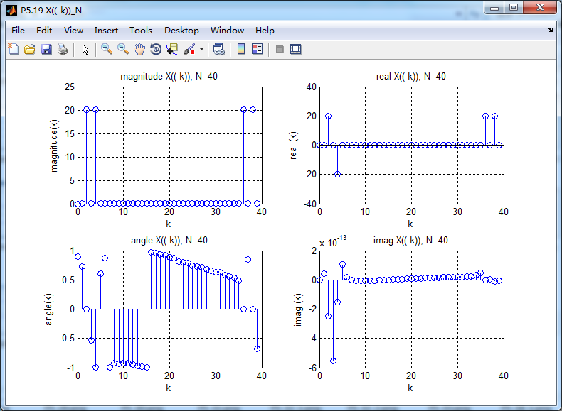
X((-k))

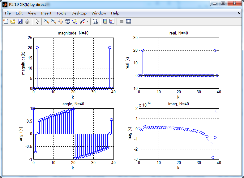
直接计算实部和虚部的DFT，XR(k)和XI(k)

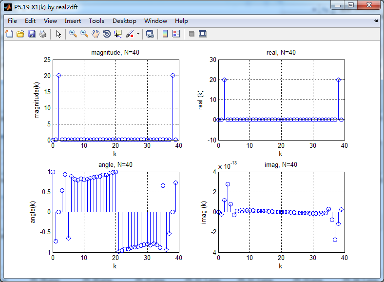
利用函数real2dft计算实部和虚部对应的DFT，Xccs(k)和Xcca(k)

结论：

如果X(k)是N点复数序列x(n)的N点DFT，x(n)=xR(n)+jxI(n)，那么有

DFT[xR]=Xccs(k)   DFT[j*xI]=Xcca(k)

实部序列的DFT是复数序列的DFT的共轭圆周对称分量

虚部序列的DFT是复数序列的DFT的共轭圆周反对称分量。