
《DSP using MATLAB》Problem 7.16
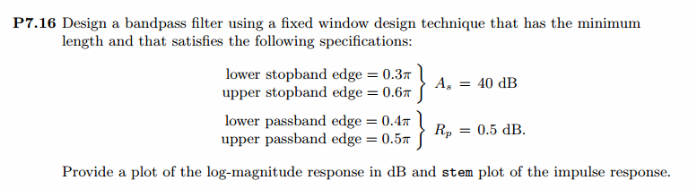
使用一种固定窗函数法设计带通滤波器。
代码:
%% ++++++++++++++++++++++++++++++++++++++++++++++++++++++++++++++++++++++++++++++++

%%            Output Info about this m-file

fprintf('\n***********************************************************\n');

fprintf('        <DSP using MATLAB> Problem 7.16 \n\n');

banner();

%% ++++++++++++++++++++++++++++++++++++++++++++++++++++++++++++++++++++++++++++++++

% bandpass

ws1 = 0.3*pi; wp1 = 0.4*pi; wp2 = 0.5*pi; ws2 = 0.6*pi; As = 40; Rp = 0.5;

tr_width = min((wp1-ws1), (ws2-wp2));

[delta1_ori, delta2_ori] = db2delta(Rp, As)

%% ---------------------------------------------------

%%         1  Rectangular Window

%% ---------------------------------------------------

M = ceil(1.8*pi/tr_width) + 1;                 % Rectangular Window

fprintf('\n\n#1.Rectangular Window, Filter Length M=%d.\n', M);

n = [0:1:M-1]; wc1 = (ws1+wp1)/2; wc2 = (wp2+ws2)/2;

hd = ideal_lp(wc2, M) - ideal_lp(wc1, M);

w_rect = (boxcar(M))';  h = hd .* w_rect;

[db, mag, pha, grd, w] = freqz_m(h, [1]);  delta_w = 2*pi/1000;

[Hr,ww,P,L] = ampl_res(h);

Rp = -(min(db(wp1/delta_w+1 :1: floor(wp2/delta_w)+1)));     % Actual Passband Ripple

fprintf('\nActual Passband Ripple is %.4f dB.\n', Rp);

As = -round(max(db(ws2/delta_w+1 : 1 : 501)));        % Min Stopband attenuation

fprintf('\nMin Stopband attenuation is %.4f dB.\n', As);

[delta1_rect, delta2_rect] = db2delta(Rp, As)

%%  ----------------------------

%%             Plot

%% -----------------------------

figure('NumberTitle', 'off', 'Name', 'Problem 7.16.1 ideal_lp Method')

set(gcf,'Color','white');

subplot(2,2,1); stem(n, hd); axis([0 M-1 -0.3 0.3]); grid on;

xlabel('n'); ylabel('hd(n)'); title('Ideal Impulse Response');

subplot(2,2,2); stem(n, w_rect); axis([0 M-1 0 1.1]); grid on;

xlabel('n'); ylabel('w(n)'); title('Rectangular Window, M=19');

subplot(2,2,3); stem(n, h); axis([0 M-1 -0.3 0.3]); grid on;

xlabel('n'); ylabel('h(n)'); title('Actual Impulse Response');

subplot(2,2,4); plot(w/pi, db); axis([0 1 -100 10]); grid on;

set(gca,'YTickMode','manual','YTick',[-90,-26,0]);

set(gca,'YTickLabelMode','manual','YTickLabel',['90';'26';' 0']);

set(gca,'XTickMode','manual','XTick',[0,0.3,0.4,0.5,0.6,1]);

xlabel('frequency in \pi units'); ylabel('Decibels'); title('Magnitude Response in dB');

figure('NumberTitle', 'off', 'Name', 'Problem 7.16.1 h(n) ideal_lp Method')

set(gcf,'Color','white');

subplot(2,2,1); plot(w/pi, db); grid on; %axis([0 1 -100 10]);

xlabel('frequency in \pi units'); ylabel('Decibels'); title('Magnitude Response in dB');

set(gca,'YTickMode','manual','YTick',[-90,-26,0])

set(gca,'YTickLabelMode','manual','YTickLabel',['90';'26';' 0']);

set(gca,'XTickMode','manual','XTick',[0,0.3,0.4,0.5,0.6,1,1.4,1.5,1.6,1.7,2]);

subplot(2,2,3); plot(w/pi, mag); grid on; %axis([0 1 -100 10]);

xlabel('frequency in \pi units'); ylabel('Absolute'); title('Magnitude Response in absolute');

set(gca,'XTickMode','manual','XTick',[0,0.3,0.4,0.5,0.6,1,1.4,1.5,1.6,1.7,2]);

set(gca,'YTickMode','manual','YTick',[0.0,0.5,1.0])

subplot(2,2,2); plot(w/pi, pha); grid on; %axis([0 1 -100 10]);

xlabel('frequency in \pi units'); ylabel('Rad'); title('Phase Response in Radians');

subplot(2,2,4); plot(w/pi, grd*pi/180);  grid on; %axis([0 1 -100 10]);

xlabel('frequency in \pi units'); ylabel('Rad'); title('Group Delay');

figure('NumberTitle', 'off', 'Name', 'Problem 7.16.1 h(n)')

set(gcf,'Color','white');

plot(ww/pi, Hr); grid on; %axis([0 1 -100 10]);

xlabel('frequency in \pi units'); ylabel('Hr'); title('Amplitude Response');

set(gca,'YTickMode','manual','YTick',[-delta2_rect,0,delta2_rect,1 - delta1_rect,1, 1 + delta1_rect])

%% ---------------------------------------------------

%%             2  Bartlett Window

%% ---------------------------------------------------

M = ceil(6.1*pi/tr_width) + 1;                 % Bartlett Window

fprintf('\n\n#2.Bartlett Window, Filter Length M=%d.\n', M);

n = [0:1:M-1]; wc1 = (ws1+wp1)/2; wc2 = (wp2+ws2)/2;

%wc = (ws + wp)/2,                    % ideal LPF cutoff frequency

hd = ideal_lp(wc2, M) - ideal_lp(wc1, M);

w_bart = (bartlett(M))';  h = hd .* w_bart;

[db, mag, pha, grd, w] = freqz_m(h, [1]);  delta_w = 2*pi/1000;

[Hr,ww,P,L] = ampl_res(h);

Rp = -(min(db(wp1/delta_w+1 :1: floor(wp2/delta_w)+1)));     % Actual Passband Ripple

fprintf('\nActual Passband Ripple is %.4f dB.\n', Rp);

As = -round(max(db(ws2/delta_w+1 : 1 : 501)));               % Min Stopband attenuation

fprintf('\nMin Stopband attenuation is %.4f dB.\n', As);

[delta1_bart, delta2_bart] = db2delta(Rp, As)

%% --------------------------

%%            Plot

%% --------------------------

figure('NumberTitle', 'off', 'Name', 'Problem 7.16.2 ideal_lp Method')

set(gcf,'Color','white');

subplot(2,2,1); stem(n, hd); axis([0 M-1 -0.2 0.2]); grid on;

xlabel('n'); ylabel('hd(n)'); title('Ideal Impulse Response');

subplot(2,2,2); stem(n, w_bart); axis([0 M-1 0 1.1]); grid on;

xlabel('n'); ylabel('w(n)'); title('Bartlett Window, M=62');

subplot(2,2,3); stem(n, h); axis([0 M-1 -0.2 0.2]); grid on;

xlabel('n'); ylabel('h(n)'); title('Actual Impulse Response');

subplot(2,2,4); plot(w/pi, db); axis([0 1 -100 10]); grid on;

set(gca,'YTickMode','manual','YTick',[-90,-27,0]);

set(gca,'YTickLabelMode','manual','YTickLabel',['90';'27';' 0']);

set(gca,'XTickMode','manual','XTick',[0,0.3,0.4,0.5,0.6,1]);

xlabel('frequency in \pi units'); ylabel('Decibels'); title('Magnitude Response in dB');

figure('NumberTitle', 'off', 'Name', 'Problem 7.16.2 h(n) ideal_lp Method')

set(gcf,'Color','white');

subplot(2,2,1); plot(w/pi, db); grid on; axis([0 2 -100 10]);

xlabel('frequency in \pi units'); ylabel('Decibels'); title('Magnitude Response in dB');

set(gca,'YTickMode','manual','YTick',[-90,-27,0])

set(gca,'YTickLabelMode','manual','YTickLabel',['90';'27';' 0']);

set(gca,'XTickMode','manual','XTick',[0,0.3,0.4,0.5,0.6,1,1.4,1.5,1.6,1.7,2]);

subplot(2,2,3); plot(w/pi, mag); grid on; %axis([0 2 -100 10]);

xlabel('frequency in \pi units'); ylabel('Absolute'); title('Magnitude Response in absolute');

set(gca,'XTickMode','manual','XTick',[0,0.3,0.4,0.5,0.6,1,1.4,1.5,1.6,1.7,2]);

set(gca,'YTickMode','manual','YTick',[0.0,0.5,1.0])

subplot(2,2,2); plot(w/pi, pha); grid on; %axis([0 1 -100 10]);

xlabel('frequency in \pi units'); ylabel('Rad'); title('Phase Response in Radians');

subplot(2,2,4); plot(w/pi, grd*pi/180);  grid on; %axis([0 1 -100 10]);

xlabel('frequency in \pi units'); ylabel('Rad'); title('Group Delay');

figure('NumberTitle', 'off', 'Name', 'Problem 7.16.2 h(n)')

set(gcf,'Color','white');

plot(ww/pi, Hr); grid on; %axis([0 1 -100 10]);

xlabel('frequency in \pi units'); ylabel('Hr'); title('Amplitude Response');

set(gca,'YTickMode','manual','YTick',[-delta2_bart,0,delta2_bart,1-delta1_bart,1, 1+delta1_bart])

%% ---------------------------------------------------

%%              3  Hann Window

%% ---------------------------------------------------

M = ceil(6.2*pi/tr_width) + 1;                 % Hann Window

fprintf('\n\n#3.Hann Window, Filter Length M=%4d.\n', M);

n = [0:1:M-1]; wc1 = (ws1+wp1)/2; wc2 = (wp2+ws2)/2;

%wc = (ws + wp)/2,                    % ideal LPF cutoff frequency

hd = ideal_lp(wc2, M) - ideal_lp(wc1, M);

w_hann = (hann(M))';  h = hd .* w_hann;

[db, mag, pha, grd, w] = freqz_m(h, [1]);  delta_w = 2*pi/1000;

[Hr,ww,P,L] = ampl_res(h);

Rp = -(min(db(wp1/delta_w+1 :1: floor(wp2/delta_w)+1)));     % Actual Passband Ripple

fprintf('\nActual Passband Ripple is %.4f dB.\n', Rp);

As = -round(max(db(ws2/delta_w+1 : 1 : 501)));               % Min Stopband attenuation

fprintf('\nMin Stopband attenuation is %.4f dB.\n', As);

[delta1_hann, delta2_hann] = db2delta(Rp, As)

%% --------------------------

%%            Plot

%% --------------------------

figure('NumberTitle', 'off', 'Name', 'Problem 7.16.3 ideal_lp Method')

set(gcf,'Color','white');

subplot(2,2,1); stem(n, hd); axis([0 M-1 -0.2 0.3]); grid on;

xlabel('n'); ylabel('hd(n)'); title('Ideal Impulse Response');

subplot(2,2,2); stem(n, w_hann); axis([0 M-1 0 1.1]); grid on;

xlabel('n'); ylabel('w(n)'); title('Hann Window, M=63');

subplot(2,2,3); stem(n, h); axis([0 M-1 -0.2 0.3]); grid on;

xlabel('n'); ylabel('h(n)'); title('Actual Impulse Response');

subplot(2,2,4); plot(w/pi, db); axis([0 1 -100 10]); grid on;

set(gca,'YTickMode','manual','YTick',[-90,-43,0]);

set(gca,'YTickLabelMode','manual','YTickLabel',['90';'43';' 0']);

set(gca,'XTickMode','manual','XTick',[0,0.3,0.4,0.5,0.6,1]);

xlabel('frequency in \pi units'); ylabel('Decibels'); title('Magnitude Response in dB');

figure('NumberTitle', 'off', 'Name', 'Problem 7.16.3 h(n) ideal_lp Method')

set(gcf,'Color','white');

subplot(2,2,1); plot(w/pi, db); grid on; axis([0 2 -100 10]);

xlabel('frequency in \pi units'); ylabel('Decibels'); title('Magnitude Response in dB');

set(gca,'YTickMode','manual','YTick',[-90,-43,0])

set(gca,'YTickLabelMode','manual','YTickLabel',['90';'43';' 0']);

set(gca,'XTickMode','manual','XTick',[0,0.3,0.4,0.5,0.6,1,1.4,1.5,1.6,1.7,2]);

subplot(2,2,3); plot(w/pi, mag); grid on; %axis([0 2 -100 10]);

xlabel('frequency in \pi units'); ylabel('Absolute'); title('Magnitude Response in absolute');

set(gca,'XTickMode','manual','XTick',[0,0.3,0.4,0.5,0.6,1,1.4,1.5,1.6,1.7,2]);

set(gca,'YTickMode','manual','YTick',[0.0,0.5,1.0])

subplot(2,2,2); plot(w/pi, pha); grid on; %axis([0 1 -100 10]);

xlabel('frequency in \pi units'); ylabel('Rad'); title('Phase Response in Radians');

subplot(2,2,4); plot(w/pi, grd*pi/180);  grid on; %axis([0 1 -100 10]);

xlabel('frequency in \pi units'); ylabel('Rad'); title('Group Delay');

figure('NumberTitle', 'off', 'Name', 'Problem 7.16.3 h(n)')

set(gcf,'Color','white');

plot(ww/pi, Hr); grid on; %axis([0 1 -100 10]);

xlabel('frequency in \pi units'); ylabel('Hr'); title('Amplitude Response');

set(gca,'YTickMode','manual','YTick',[-delta2_hann,0,delta2_hann,1 - delta1_hann,1, 1 + delta1_hann])

%% ---------------------------------------------------

%%             4  Hamming Window

%% ---------------------------------------------------

M = ceil(6.6*pi/tr_width) + 1;                 % Hamming Window

fprintf('\n\n#4.Hamming Window, Filter Length M=%4d.\n', M);

n = [0:1:M-1]; wc1 = (ws1+wp1)/2; wc2 = (wp2+ws2)/2;

%wc = (ws + wp)/2,                    % ideal LPF cutoff frequency

hd = ideal_lp(wc2, M) - ideal_lp(wc1, M);

w_hamm = (hamming(M))';  h = hd .* w_hamm;

[db, mag, pha, grd, w] = freqz_m(h, [1]);  delta_w = 2*pi/1000;

[Hr,ww,P,L] = ampl_res(h);

Rp = -(min(db(wp1/delta_w+1 :1: floor(wp2/delta_w)+1)));     % Actual Passband Ripple

fprintf('\nActual Passband Ripple is %.4f dB.\n', Rp);

As = -round(max(db(ws2/delta_w+1 : 1 : 501)));               % Min Stopband attenuation

fprintf('\nMin Stopband attenuation is %.4f dB.\n', As);

[delta1_hamm, delta2_hamm] = db2delta(Rp, As)

%% --------------------------

%%            Plot

%% --------------------------

figure('NumberTitle', 'off', 'Name', 'Problem 7.16.4 ideal_lp Method')

set(gcf,'Color','white');

subplot(2,2,1); stem(n, hd); axis([0 M-1 -0.2 0.3]); grid on;

xlabel('n'); ylabel('hd(n)'); title('Ideal Impulse Response');

subplot(2,2,2); stem(n, w_hamm); axis([0 M-1 0 1.1]); grid on;

xlabel('n'); ylabel('w(n)'); title('Hamming Window, M=67');

subplot(2,2,3); stem(n, h); axis([0 M-1 -0.2 0.3]); grid on;

xlabel('n'); ylabel('h(n)'); title('Actual Impulse Response');

subplot(2,2,4); plot(w/pi, db); axis([0 1 -100 10]); grid on;

set(gca,'YTickMode','manual','YTick',[-90,-51,0]);

set(gca,'YTickLabelMode','manual','YTickLabel',['90';'51';' 0']);

set(gca,'XTickMode','manual','XTick',[0,0.3,0.4,0.5,0.6,1]);

xlabel('frequency in \pi units'); ylabel('Decibels'); title('Magnitude Response in dB');

figure('NumberTitle', 'off', 'Name', 'Problem 7.16.4 h(n) ideal_lp Method')

set(gcf,'Color','white');

subplot(2,2,1); plot(w/pi, db); grid on; axis([0 2 -100 10]);

xlabel('frequency in \pi units'); ylabel('Decibels'); title('Magnitude Response in dB');

set(gca,'YTickMode','manual','YTick',[-90,-51,0])

set(gca,'YTickLabelMode','manual','YTickLabel',['90';'51';' 0']);

set(gca,'XTickMode','manual','XTick',[0,0.3,0.4,0.5,0.6,1,1.4,1.5,1.6,1.7,2]);

subplot(2,2,3); plot(w/pi, mag); grid on; %axis([0 2 -100 10]);

xlabel('frequency in \pi units'); ylabel('Absolute'); title('Magnitude Response in absolute');

set(gca,'XTickMode','manual','XTick',[0,0.3,0.4,0.5,0.6,1,1.4,1.5,1.6,1.7,2]);

set(gca,'YTickMode','manual','YTick',[0.0,0.5,1.0])

subplot(2,2,2); plot(w/pi, pha); grid on; %axis([0 1 -100 10]);

xlabel('frequency in \pi units'); ylabel('Rad'); title('Phase Response in Radians');

subplot(2,2,4); plot(w/pi, grd*pi/180);  grid on; %axis([0 1 -100 10]);

xlabel('frequency in \pi units'); ylabel('Rad'); title('Group Delay');

figure('NumberTitle', 'off', 'Name', 'Problem 7.16.4 h(n)')

set(gcf,'Color','white');

plot(ww/pi, Hr); grid on; %axis([0 1 -100 10]);

xlabel('frequency in \pi units'); ylabel('Hr'); title('Amplitude Response');

set(gca,'YTickMode','manual','YTick',[-delta2_hamm,0,delta2_hamm,1 - delta1_hamm,1, 1 + delta1_hamm])

%% ---------------------------------------------------

%%             5  Blackman Window

%% ---------------------------------------------------

M = ceil(11*pi/tr_width) + 1;                 % Blackman Window

fprintf('\n\n#5.Blackman Window, Filter Length M=%d.\n', M);

n = [0:1:M-1]; wc1 = (ws1+wp1)/2; wc2 = (wp2+ws2)/2;

%wc = (ws + wp)/2,                    % ideal LPF cutoff frequency

hd = ideal_lp(wc2, M) - ideal_lp(wc1, M);

w_bla = (blackman(M))';  h = hd .* w_bla;

[db, mag, pha, grd, w] = freqz_m(h, [1]);  delta_w = 2*pi/1000;

[Hr,ww,P,L] = ampl_res(h);

Rp = -(min(db(wp1/delta_w+1 :1: floor(wp2/delta_w)+1)));     % Actual Passband Ripple

fprintf('\nActual Passband Ripple is %.4f dB.\n', Rp);

As = -round(max(db(ws2/delta_w+1 : 1 : 501)));               % Min Stopband attenuation

fprintf('\nMin Stopband attenuation is %.4f dB.\n', As);

[delta1_bla, delta2_bla] = db2delta(Rp, As)

%% --------------------------

%%            Plot

%% --------------------------

figure('NumberTitle', 'off', 'Name', 'Problem 7.16.5 ideal_lp Method')

set(gcf,'Color','white');

subplot(2,2,1); stem(n, hd); axis([0 M-1 -0.2 0.3]); grid on;

xlabel('n'); ylabel('hd(n)'); title('Ideal Impulse Response');

subplot(2,2,2); stem(n, w_bla); axis([0 M-1 0 1.1]); grid on;

xlabel('n'); ylabel('w(n)'); title('Blackman Window, M=111');

subplot(2,2,3); stem(n, h); axis([0 M-1 -0.2 0.3]); grid on;

xlabel('n'); ylabel('h(n)'); title('Actual Impulse Response');

subplot(2,2,4); plot(w/pi, db); axis([0 1 -120 10]); grid on;

set(gca,'YTickMode','manual','YTick',[-90,-73,0]);

set(gca,'YTickLabelMode','manual','YTickLabel',['90';'73';' 0']);

set(gca,'XTickMode','manual','XTick',[0,0.3,0.4,0.5,0.6,1]);

xlabel('frequency in \pi units'); ylabel('Decibels'); title('Magnitude Response in dB');

figure('NumberTitle', 'off', 'Name', 'Problem 7.16.5 h(n) ideal_lp Method')

set(gcf,'Color','white');

subplot(2,2,1); plot(w/pi, db); grid on; axis([0 2 -120 10]);

xlabel('frequency in \pi units'); ylabel('Decibels'); title('Magnitude Response in dB');

set(gca,'YTickMode','manual','YTick',[-90,-73,0])

set(gca,'YTickLabelMode','manual','YTickLabel',['90';'73';' 0']);

set(gca,'XTickMode','manual','XTick',[0,0.3,0.4,0.5,0.6,1,1.4,1.5,1.6,1.7,2]);

subplot(2,2,3); plot(w/pi, mag); grid on; %axis([0 2 -120 10]);

xlabel('frequency in \pi units'); ylabel('Absolute'); title('Magnitude Response in absolute');

set(gca,'XTickMode','manual','XTick',[0,0.3,0.4,0.5,0.6,1,1.4,1.5,1.6,1.7,2]);

set(gca,'YTickMode','manual','YTick',[0.0,0.5,1.0])

subplot(2,2,2); plot(w/pi, pha); grid on; %axis([0 1 -100 10]);

xlabel('frequency in \pi units'); ylabel('Rad'); title('Phase Response in Radians');

subplot(2,2,4); plot(w/pi, grd*pi/180);  grid on; %axis([0 1 -100 10]);

xlabel('frequency in \pi units'); ylabel('Rad'); title('Group Delay');

figure('NumberTitle', 'off', 'Name', 'Problem 7.16.5 h(n)')

set(gcf,'Color','white');

plot(ww/pi, Hr); grid on; %axis([0 1 -100 10]);

xlabel('frequency in \pi units'); ylabel('Hr'); title('Amplitude Response');

set(gca,'YTickMode','manual','YTick',[-delta2_bla,0,delta2_bla,1-delta1_bla,1, 1+delta1_bla])

%% ---------------------------------------------------

%%             6  Kaiser Window

%% ---------------------------------------------------

M = ceil((As-7.95)/(2.285*tr_width)) + 1;                 % Kaiser Window

if As > 21 || As < 50

	beta = 0.5842*(As-21)^0.4 + 0.07886*(As-21);

else

	beta = 0.1102*(As-8.7);

end

fprintf('\n\n#6.Kaiser Window, Filter Length M=%d, beta=%.4f\n', M,beta);

n = [0:1:M-1]; wc1 = (ws1+wp1)/2; wc2 = (wp2+ws2)/2;

%wc = (ws + wp)/2,                    % ideal LPF cutoff frequency

hd = ideal_lp(wc2, M) - ideal_lp(wc1, M);

w_kai = (kaiser(M,beta))';  h = hd .* w_kai;

[db, mag, pha, grd, w] = freqz_m(h, [1]);  delta_w = 2*pi/1000;

[Hr,ww,P,L] = ampl_res(h);

Rp = -(min(db(wp1/delta_w+1 :1: floor(wp2/delta_w)+1)));     % Actual Passband Ripple

fprintf('\nActual Passband Ripple is %.4f dB.\n', Rp);

As = -round(max(db(ws2/delta_w+1 : 1 : 501)));               % Min Stopband attenuation

fprintf('\nMin Stopband attenuation is %.4f dB.\n', As);

[delta1_kai, delta2_kai] = db2delta(Rp, As)

%% --------------------------

%%            Plot

%% --------------------------

figure('NumberTitle', 'off', 'Name', 'Problem 7.16.6 ideal_lp Method')

set(gcf,'Color','white');

subplot(2,2,1); stem(n, hd); axis([0 M-1 -0.2 0.2]); grid on;

xlabel('n'); ylabel('hd(n)'); title('Ideal Impulse Response');

subplot(2,2,2); stem(n, w_kai); axis([0 M-1 0 1.1]); grid on;

xlabel('n'); ylabel('w(n)'); title('Kaiser Window, M=92');

subplot(2,2,3); stem(n, h); axis([0 M-1 -0.2 0.2]); grid on;

xlabel('n'); ylabel('h(n)'); title('Actual Impulse Response');

subplot(2,2,4); plot(w/pi, db); axis([0 1 -120 10]); grid on;

set(gca,'YTickMode','manual','YTick',[-90,-72,0]);

set(gca,'YTickLabelMode','manual','YTickLabel',['90';'72';' 0']);

set(gca,'XTickMode','manual','XTick',[0,0.3,0.4,0.5,0.6,1]);

xlabel('frequency in \pi units'); ylabel('Decibels'); title('Magnitude Response in dB');

figure('NumberTitle', 'off', 'Name', 'Problem 7.16.6 h(n) ideal_lp Method')

set(gcf,'Color','white');

subplot(2,2,1); plot(w/pi, db); grid on; axis([0 2 -120 10]);

xlabel('frequency in \pi units'); ylabel('Decibels'); title('Magnitude Response in dB');

set(gca,'YTickMode','manual','YTick',[-90,-72,0])

set(gca,'YTickLabelMode','manual','YTickLabel',['90';'72';' 0']);

set(gca,'XTickMode','manual','XTick',[0,0.3,0.4,0.5,0.6,1,1.4,1.5,1.6,1.7,2]);

subplot(2,2,3); plot(w/pi, mag); grid on; %axis([0 2 -100 10]);

xlabel('frequency in \pi units'); ylabel('Absolute'); title('Magnitude Response in absolute');

set(gca,'XTickMode','manual','XTick',[0,0.3,0.4,0.5,0.6,1,1.4,1.5,1.6,1.7,2]);

set(gca,'YTickMode','manual','YTick',[0.0,0.5,1.0])

subplot(2,2,2); plot(w/pi, pha); grid on; %axis([0 1 -100 10]);

xlabel('frequency in \pi units'); ylabel('Rad'); title('Phase Response in Radians');

subplot(2,2,4); plot(w/pi, grd*pi/180);  grid on; %axis([0 1 -100 10]);

xlabel('frequency in \pi units'); ylabel('Rad'); title('Group Delay');

figure('NumberTitle', 'off', 'Name', 'Problem 7.16.6 h(n)')

set(gcf,'Color','white');

plot(ww/pi, Hr); grid on; %axis([0 1 -100 10]);

xlabel('frequency in \pi units'); ylabel('Hr'); title('Amplitude Response');

set(gca,'YTickMode','manual','YTick',[-delta2_kai,0,delta2_kai,1-delta1_kai,1, 1+delta1_kai])
运行结果:
设计指标,As=40dB,Rp=0.5dB;换算成绝对指标,为δ1=0.0288,δ2=0.0103。

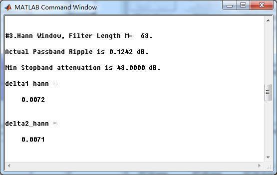
由书中表7.1可知,矩形窗(Rectangular)和三角窗(Bartlett)不满足设计要求,这里我们也进行贴图验证。


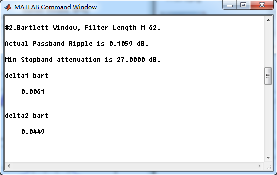

上图可知,rectangualr窗和bartlett窗不符合设计要求。
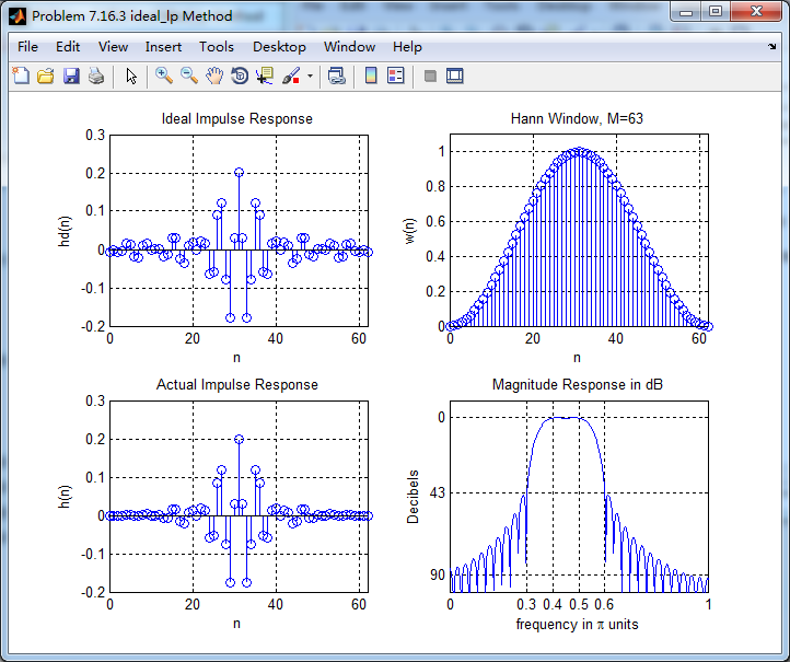

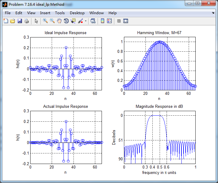

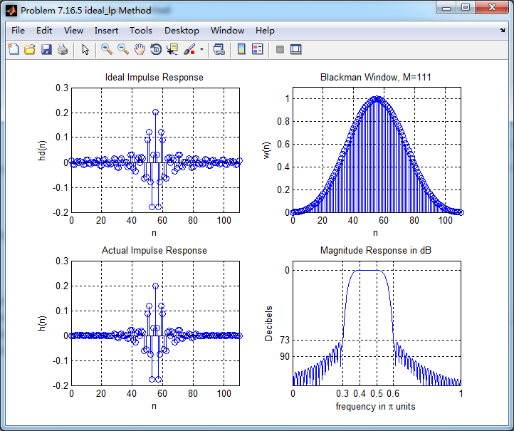

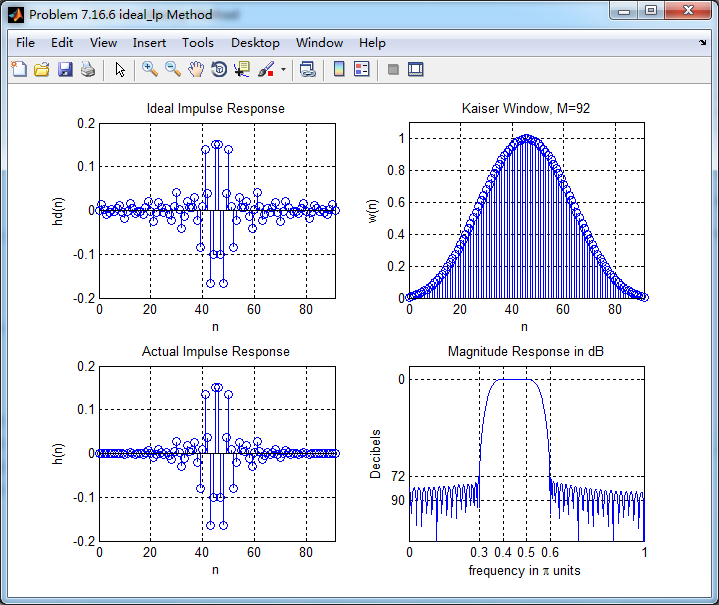
下面将以上几种窗函数设计结果,总结如下
| 序号 | 名 称 | 长度M | As | Rp |
| 1 | Rectangular | 19 | 26 | 1.918 |
| 2 | Bartlett | 62 | 27 | 0.1059 |
| 3 | Hann | 63 | 43 | 0.1242 |
| 4 | Hamming | 67 | 51 | 0.0488 |
| 5 | Blackman | 111 | 73 | 0.0027 |
| 6 | Kaiser | 92 | 72 | 0.0049 |
由上表得知,满足设计要求的是用长M=63的Hann窗截断得到的滤波器。
《DSP using MATLAB》Problem 7.16的更多相关文章
- 《DSP using MATLAB》Problem 4.16
代码: %% ------------------------------------------------------------------------ %% Output Info about ...
- 《DSP using MATLAB》Problem 2.16
先由脉冲响应序列h(n)得到差分方程系数,过程如下: 代码: %% ------------------------------------------------------------------ ...
- 《DSP using MATLAB》Problem 6.16
从别的地方找来的: 截图有些乱. 结构流程图如下
- 《DSP using MATLAB》Problem 7.26
注意:高通的线性相位FIR滤波器,不能是第2类,所以其长度必须为奇数.这里取M=31,过渡带里采样值抄书上的. 代码: %% +++++++++++++++++++++++++++++++++++++ ...
- 《DSP using MATLAB》Problem 5.10
代码: 第1小题: %% ++++++++++++++++++++++++++++++++++++++++++++++++++++++++++++++++++++++++++++++++ %% Out ...
- 《DSP using MATLAB》Problem 4.11
代码: %% ---------------------------------------------------------------------------- %% Output Info a ...
- 《DSP using MATLAB》Problem 9.2
前几天看了看博客,从16年底到现在,3年了,终于看书到第9章了.都怪自己愚钝不堪,唯有吃苦努力,一点一点一页一页慢慢啃了. 代码: %% ------------------------------- ...
- 《DSP using MATLAB》Problem 8.31
代码: %% ------------------------------------------------------------------------ %% Output Info about ...
- 《DSP using MATLAB》Problem 8.29
来汉有一月,往日的高温由于最近几个台风沿海登陆影响,今天终于下雨了,凉爽了几个小时. 接着做题. %% ------------------------------------------------ ...
随机推荐
- 关注Yumiot公众号,了解最新的物联网资讯
Yumiot,专注于物联网行业,每天不定期推送最新的物联网行业新闻.详情请用微信搜索关注 yumiot .
- 简要log4j配置
若排版紊乱可查看我的个人博客原文地址 1. 配置效果 下面的log4j日志配置最终能达到的效果是对于全局日志可以根据级别输入到对应级别的日志文件中,注意低级别的日志文件会同时包含高级别的日志信息,例如 ...
- my goal
I want to get a good command of a programming language at the university, and I have to pass the tes ...
- java——形参与实参
看了很多的文章,稍微有一些的总结:对最基本的形参与实参有了一定的理解,虽然还是不够深入. 1.基本概念 形参:全称为"形式参数"是在定义函数名和函数体的时候使用的参数,目的是用来接 ...
- Atom本地安装插件右上角出现红色报错解决方案
在github上搜索你相中的插件(Package),并下载ZIP包或直接克隆项目到本地.然后将该包直接复制到C盘中的用户下的 .atom\packages\ 文件夹下,注意 atom前面有一个点. 然 ...
- Linux系统调用列表(转)
以下是Linux系统调用的一个列表,包含了大部分常用系统调用和由系统调用派生出的的函数.这可能是你在互联网上所能看到的唯一一篇中文注释的Linux系统调用列表,即使是简单的字母序英文列表,能做到这么完 ...
- json格式字符串用Uncaught SyntaxError: Unexpected token ' Uncaught SyntaxError: Unexpected number
Unexpected number(index)的错误用的json字符串如 var jsonStr = "{1:'北京note备注信息',2:'上海note备注信息',3:'广东note备注 ...
- linux的ls命令中文件颜色含义
linux命令ls会显示出文件的颜色, 系统约定的默认颜色含义如下: 白色:表示普通文件 蓝色:表示目录 绿色:表示可执行文件 红色:表示压缩文件 浅蓝色:链接文件 主要是使用ln命令建立的文件 红色 ...
- 2016/12/21 dplの课练
1.将/etc/passwd第行的最后一段全部改成/bin/bash cat 1 |sed -n '1,$p' |egrep '.*:' -o |sed 's/$/\bin\/bash/' 2.将/e ...
- C++的qsort函数
void qsort(void * base,int nelem,int width,int (*fcmp)(const void*,const void *) 1.待排序数组首地址 2.数组中待排序 ...