7. The Singular Value Decomposition(SVD)

7.1 Singular values and Singular vectors

The SVD separates any matrix into simple pieces.

A is any m by n matrix, square or rectangular, Its rank is r.

Choices from the SVD

\[AA^Tu_i = \sigma_i^{2}u_i \\
A^TAv_i = \sigma_i^{2}v_i \\
Av_i = \sigma_i u_i
\]

$u_i$— the left singular vectors (unit eigenvectors of $AA^T$)

$v_i$— the right singular vectors (unit eigenvectors of $A^TA$)

$\sigma_i$— singular values (square roots of the equal eigenvalues of $AA^T$ and $A^TA$)

The rank of A is equal to numbers of $\sigma _i$

example:

\[A = \left [ \begin{matrix} 1&0 \\ 1&1 \end{matrix}\right] \\
\Downarrow \\
AA^T =
\left [ \begin{matrix} 1&0 \\ 1&1 \end{matrix}\right]
\left [ \begin{matrix} 1&1 \\ 0&1 \end{matrix}\right]
=\left [ \begin{matrix} 1&1 \\ 1&2 \end{matrix}\right]
\\
A^TA =
\left [ \begin{matrix} 1&1 \\ 0&1 \end{matrix}\right]
\left [ \begin{matrix} 1&0 \\ 1&1 \end{matrix}\right]
=\left [ \begin{matrix} 2&1 \\ 1&1 \end{matrix}\right]
\\
\Downarrow \\
det(AA^T - I) = 0 \ \quad \ det(A^TA - I) = 0 \\
\lambda_1 = \frac{3+\sqrt{5}}{2} , \sigma_1=\frac{1+\sqrt{5}}{2},
u_1= \frac{1}{\sqrt{1+\sigma_1^2}}\left [ \begin{matrix} 1 \\ \sigma_1 \end{matrix}\right],
v_1= \frac{1}{\sqrt{1+\sigma_1^2}}\left [ \begin{matrix} \sigma_1 \\ 1 \end{matrix}\right]
\\
\lambda_2 = \frac{3-\sqrt{5}}{2} , \sigma_1=\frac{1-\sqrt{5}}{2},
u_2= \frac{1}{\sqrt{1+\sigma_2^2}}\left [ \begin{matrix} \sigma_1 \\ -1 \end{matrix}\right],
v_2= \frac{1}{\sqrt{1+\sigma_2^2}}\left [ \begin{matrix} 1 \\ -\sigma_1 \end{matrix}\right]\\
\Downarrow \\
A =
\left [ \begin{matrix} u_1&u_2 \end{matrix}\right]
\left [ \begin{matrix} \sigma_1&\\&\sigma_2 \end{matrix}\right]
\left [ \begin{matrix} v_1^T\\v_2^T \end{matrix}\right]
\\
A\left [ \begin{matrix} v_1&v_2 \end{matrix}\right] =
\left [ \begin{matrix} u_1&u_2 \end{matrix}\right]
\left [ \begin{matrix} \sigma_1&\\&\sigma_2 \end{matrix}\right]
\]

7.2 Bases and Matrices in the SVD

Keys:

The SVD produces orthonormal basis of $u's$ and $ v's$ for the four fundamental subspaces.
- $u_1,u_2,...,u_r$ is an orthonormal basis of the column space. ($R^m$)
- $u_{r+1},...,u_{m}$ is an orthonormal basis of the left nullspace. ($R^m$)
- $v_1,v_2,...,v_r$ is an orthonormal basis of the row space. ($R^n$)
- $v_{r+1},...,u_{n}$ is an orthonormal basis of the nullspace.($R^n$)
Using those basis, A can be diagonalized :

Reduced SVD: only with bases for the row space and column space.

\[A = U_r \Sigma_r V_r^T \\
U = \left [ \begin{matrix} u_1&\cdots&u_r\\ \end{matrix}\right] ,
\Sigma_r = \left [ \begin{matrix} \sigma_1&&\\&\ddots&\\&&\sigma_r \end{matrix}\right],
V_r^T=\left [ \begin{matrix} v_1\\ \vdots \\ v_r \end{matrix}\right] \\
\Downarrow \\
A = \left [ \begin{matrix} u_1&\cdots&u_r\\ \end{matrix}\right]
\left [ \begin{matrix} \sigma_1&&\\&\ddots&\\&&\sigma_r \end{matrix}\right]
\left [ \begin{matrix} v_1\\ \vdots \\ v_r \end{matrix}\right] \\
= u_1\sigma_1v_{1}^T + u_2\sigma_2v_{2}^T + \cdots + u_r\sigma_rv_r^T
\]

Full SVD: include four subspaces.

\[A = U \Sigma V^T \\
U = \left [ \begin{matrix} u_1&\cdots&u_r&\cdots&u_n\\ \end{matrix}\right] ,
\Sigma_r = \left [ \begin{matrix} \sigma_1&&\\&\ddots&\\&&\sigma_r \\ &&&\ddots \\ &&&&\sigma_n \end{matrix}\right],
V^T=\left [ \begin{matrix} v_1\\ \vdots \\ v_r \\ \vdots \\ v_m \end{matrix}\right] \\
\Downarrow \\
A = \left [ \begin{matrix} u_1&\cdots&u_r&\cdots&u_n\\ \end{matrix}\right]
\left [ \begin{matrix} \sigma_1&&\\&\ddots&\\&&\sigma_r \\ &&&\ddots \\ &&&&\sigma_n \end{matrix}\right]
\left [ \begin{matrix} v_1\\ \vdots \\ v_r \\ \vdots \\ v_m \end{matrix}\right] \\
= u_1\sigma_1v_{1}^T + u_2\sigma_2v_{2}^T + \cdots + u_r\sigma_rv_r^T\cdots + u_n\sigma_n v_n^{T} + \cdots + u_m\sigma_mv_m^T
\]

example: $A=\left [ \begin{matrix} 3&0 \\ 4&5 \end{matrix}\right]$, r=2

\[A^TA =\left [ \begin{matrix} 25&20 \\ 20&25 \end{matrix}\right],
AA^T =\left [ \begin{matrix} 9&12 \\ 12&41 \end{matrix}\right] \\
\lambda_1 = 45, \sigma_1 = \sqrt{45},
v_1 = \frac{1}{\sqrt{2}}
\left [ \begin{matrix} 1 \\ 1 \end{matrix}\right],
u_1 = \frac{1}{\sqrt{10}}
\left [ \begin{matrix} 1 \\ 3 \end{matrix}\right]\\
\lambda_2 = 5, \sigma_2 = \sqrt{5} ,
v_2 = \frac{1}{\sqrt{2}}
\left [ \begin{matrix} -1 \\ 1 \end{matrix}\right],
u_2 = \frac{1}{\sqrt{10}}
\left [ \begin{matrix} -3 \\ 1 \end{matrix}\right]\\
\Downarrow \\
U = \frac{1}{\sqrt{10}}
\left [ \begin{matrix} 1&-3 \\ 3&1 \end{matrix}\right],
\Sigma = \left [ \begin{matrix} \sqrt{45}& \\ &\sqrt{5} \end{matrix}\right],
V = \frac{1}{\sqrt{2}}
\left [ \begin{matrix} 1&-1 \\ 1&1 \end{matrix}\right]
\]

7.3 The geometry of the SVD

$A = U\Sigma V^T$ factors into (rotation)(stretching)(rotation), the geometry shows how A transforms vectors x on a circle to vectors Ax on an ellipse.

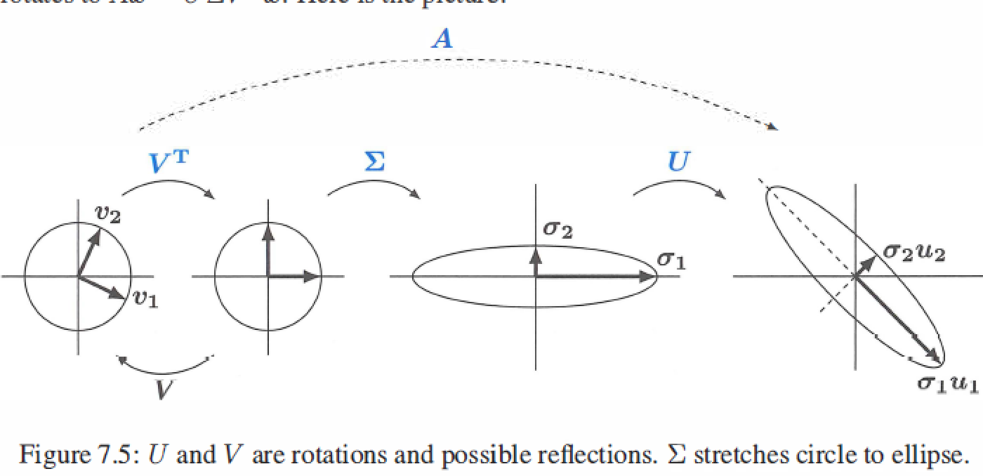
Polar decomposition factors A into QS : rotation $Q=UV^T$ times streching $S=V \Sigma V^T$.

\[V^TV = I \\
A = U\Sigma V^T = (UV^T)(V\Sigma V^T) = (Q)(S)
\]

Q is orthogonal and inclues both rotations U and $V^T$, S is symmetric positive semidefinite and gives the stretching directions.

If A is invertible, S is positive definite.
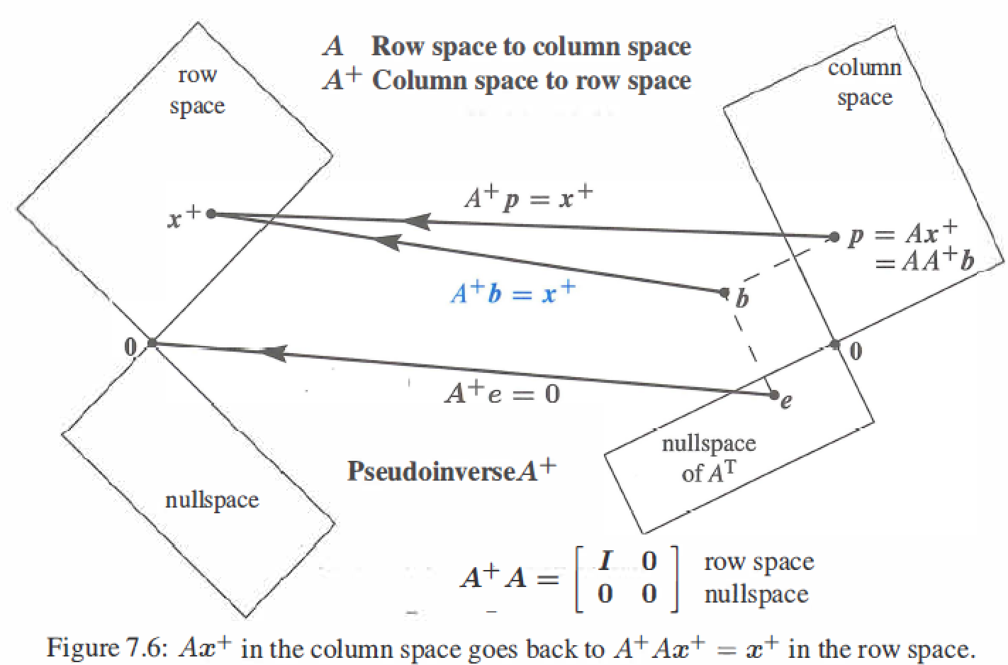
The Pseudoinverse $A^{+}: AA^{+}=I$
- $Av_i=\sigma_iu_i$ : A multiplies $v_i$ in the row space of A to give $\sigma_i u_i$ in the column space of A.
- If $A^{-1}$ exists, $A^{-1}u_i=\frac{v_i}{\sigma}$ : $A^{-1}$ multiplies $u_i$ in the row space of $A^{-1}$ to give $\sigma_i u_i$ in the column space of $A^{-1}$, $1/\sigma_i$ is singular values of $A^{-1}$.
- Pseudoinverse of A: if $A^{-1}$ exists, then $A^{+}$ is the same as $A^{-1}$
  
  \[A^{+} = V \Sigma^{+}U^{T} = \left [ \begin{matrix} v_1&\cdots&v_r&\cdots&v_n\\ \end{matrix}\right]
  \left [ \begin{matrix} \sigma_1^{-1}&&\\&\ddots&\\&&\sigma_r^{-1} \\ &&&\ddots \\ &&&&\sigma_n^{-1} \end{matrix}\right]
  \left [ \begin{matrix} u_1\\ \vdots \\ u_r \\ \vdots \\ u_m \end{matrix}\right] \\
  \]

7.4 Principal Component Analysis ( PCA by the SVD)

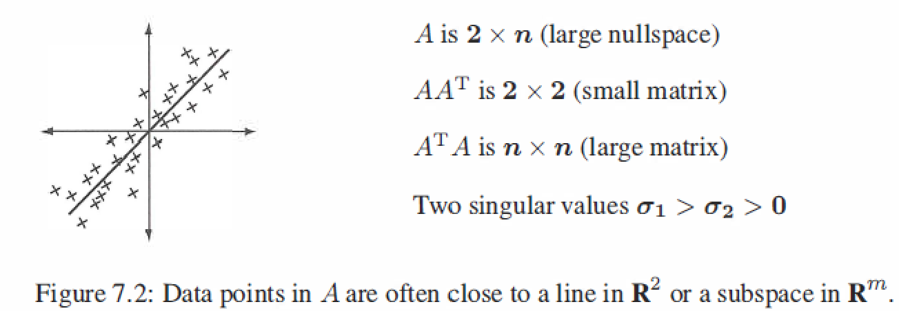
PCA gives a way to understand a data plot in dimension m, applications mostly are human genetics \ face recognition\ finance \ model order reduction (computation) .

The sample covariance matrix $S=AA^T/(n-1)$

The crucial connection to linear algebra is in the singular values and singular vectors of A, which comes from the eigenvalues $\lambda=\sigma^2$ and the eigenvectors u of the sample covariance matrix $S=AA^T/(n-1)$

The total variance in the data is the sum of all eigenvalues and of sample variances $s^2$ :

\[T = \sigma_1^2 + \cdots + \sigma_m^2 = s_1^2 + \cdots + s_m^2 = trace(diagonal \ \ sum)
\]
The first eigenvector $u_1$ of S points in the most significant direction of the data.That direction accounts for a fraction $\sigma_1^2/T$ of the total variance.
The next eigenvectors $u_2$ (orthogonal to $u_1$) accounts for a small fraction $\sigma_2^2/T$.
Stop when those fractions are small. You have the R directions that explain most of the data.The n data points are very near an R-dimensional subspace with basis $u_1, \cdots, u_R$, which are the principal components.
R is the "effective rank" of A. The true rank r is probably m or n : full rank matrix.

example: $A = \left[ \begin{matrix} 3&-4&7&-1&-4&-3 \\ 7&-6&8&-1&-1&-7 \end{matrix} \right]$ has sample covariance $S=AA^T/5 = \left [ \begin{matrix} 20&25 \\ 25&40 \end{matrix}\right]$

The eigenvalues of S are 57 and 3，so the first rank one piece $\sqrt{57}u_1v_1^T$ is much larger than the second piece $\sqrt{3}u_2v_2^T$.

The leading eigenvector $u_1 = (0.6,0.8)$ shows the direction that you see in the scatter graph.

The SVD of A (centered data) shows the dominant direction in the scatter plot.

The second eigenvector $u_2$ is perpendicular to $u_1$. The second singular value $\sigma_2=\sqrt{3}$ measures the spread across the dominant line.