吴裕雄--天生自然 R语言数据分析：火箭发射的地点、日期/时间和结果分析

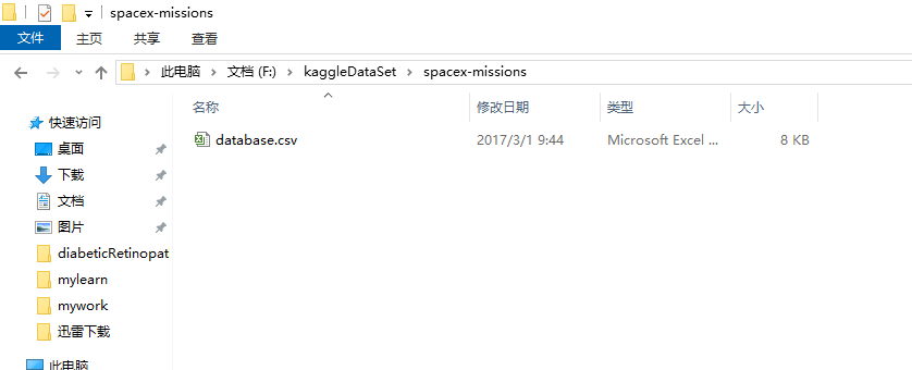
dfS = read.csv("F:\\kaggleDataSet\\spacex-missions\\database.csv")

library(dplyr)
library(tidyr)
library(data.table)
library(sqldf)
library(highcharter)
library(ggrepel)
library(leaflet)
library(viridisLite)
library(countrycode)
library(ggplot2)

names(dfS) <- gsub("\\.", "", names(dfS))
dfS$CustomerCountry = sub(x = dfS$CustomerCountry, pattern = "France (Mexico)", replacement = "France", fixed=T)

dfS = data.table(sqldf(c("UPDATE dfS SET PayloadType = PayloadName WHERE PayloadType == ''",
                            "SELECT * FROM main.dfS"), method = "raw"))
dfS = data.table(sqldf(c("UPDATE dfS SET PayloadOrbit = 'Unknown' WHERE PayloadOrbit == ''",
                            "SELECT * FROM main.dfS"), method = "raw"))
dfS = data.table(sqldf(c("UPDATE dfS SET CustomerName = 'N/A' WHERE CustomerName == ''", "SELECT * FROM main.dfS"),
                       method = "raw"))
dfS = data.table(sqldf(c("UPDATE dfS SET CustomerType = 'N/A' WHERE CustomerType == ''", "SELECT * FROM main.dfS"),
                       method = "raw"))
dfS = data.table(sqldf(c("UPDATE dfS SET CustomerCountry = 'N/A'WHERE CustomerCountry == ''",
                            "SELECT * FROM main.dfS"), method = "raw"))
dfS$PayloadMasskg[is.na(dfS$PayloadMasskg)] <- 'Unknown'

dfS = as.data.frame(dfS)
date.chr <- as.character(dfS$LaunchDate)
date <- strptime(date.chr,format="%d %b %Y")
dfS$LaunchDate = date
dfS$LaunchDate = as.Date(dfS$LaunchDate)

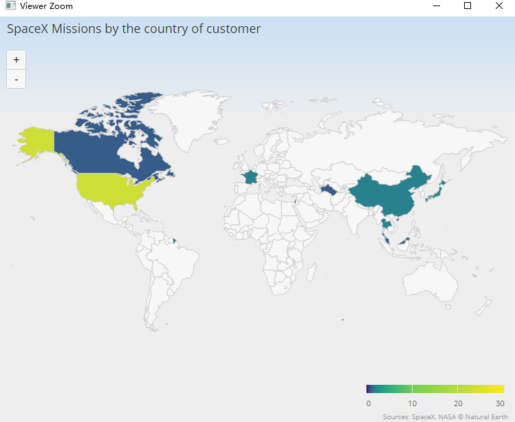
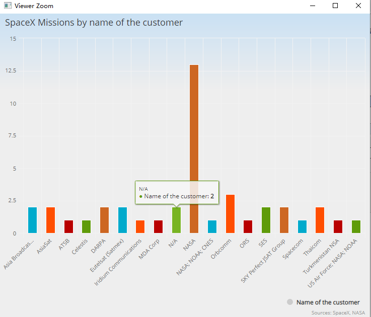
hchart(dfS$CustomerCountry, colorByPoint = TRUE, name = "Customer's country") %>%
  hc_title(text = "SpaceX Missions by the country of customer") %>% hc_add_theme(hc_theme_flat()) %>%
  hc_credits(enabled = TRUE, text = "Sources: SpaceX, NASA", style = list(fontSize = "10px"))

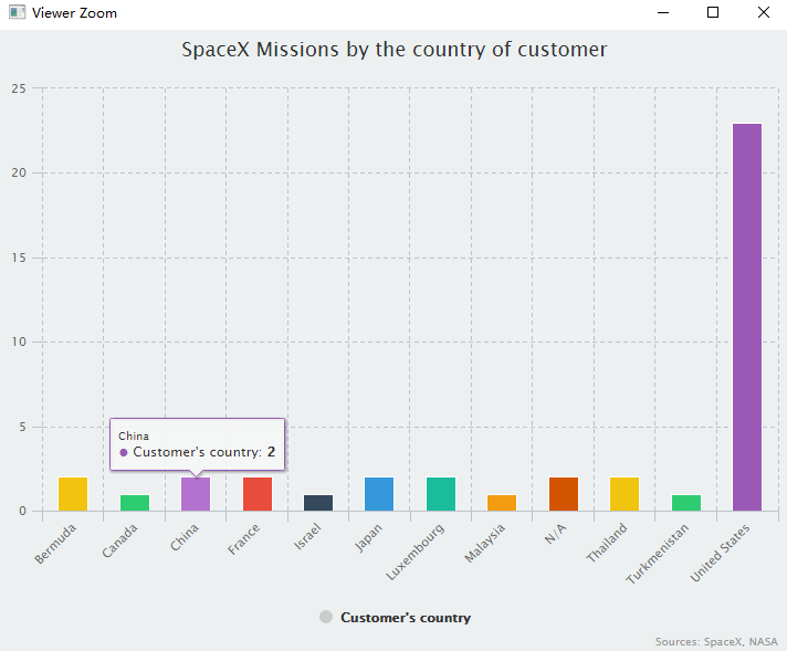
hchart(dfS$CustomerName, colorByPoint = TRUE, name = "Name of the customer") %>%
  hc_title(text = "SpaceX Missions by name of the customer") %>% hc_add_theme(hc_theme_ffx()) %>%
  hc_credits(enabled = TRUE, text = "Sources: SpaceX, NASA", style = list(fontSize = "10px"))

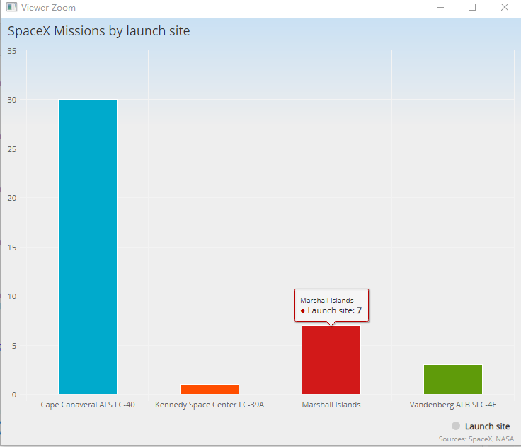
hchart(dfS$LaunchSite, colorByPoint = TRUE, name = "Launch site") %>%
  hc_title(text = "SpaceX Missions by launch site") %>% hc_add_theme(hc_theme_ffx()) %>%
  hc_credits(enabled = TRUE, text = "Sources: SpaceX, NASA", style = list(fontSize = "10px"))

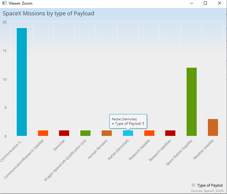
hchart(dfS$PayloadType, colorByPoint = TRUE, name = "Type of Paylod") %>%
  hc_title(text = "SpaceX Missions by type of Payload") %>% hc_add_theme(hc_theme_ffx()) %>%
  hc_credits(enabled = TRUE, text = "Sources: SpaceX, NASA", style = list(fontSize = "10px"))

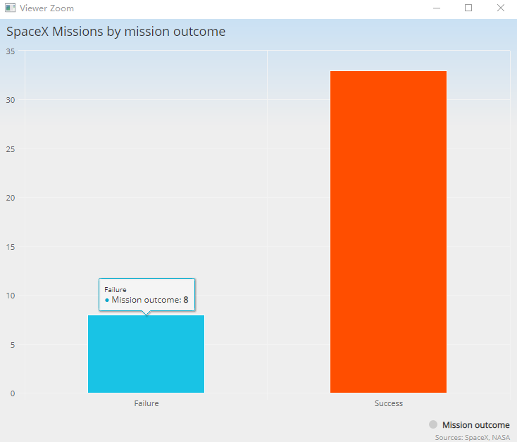
hchart(dfS$MissionOutcome, colorByPoint = TRUE, name = "Mission outcome") %>%
  hc_title(text = "SpaceX Missions by mission outcome") %>% hc_add_theme(hc_theme_ffx()) %>%
  hc_credits(enabled = TRUE, text = "Sources: SpaceX, NASA", style = list(fontSize = "10px"))

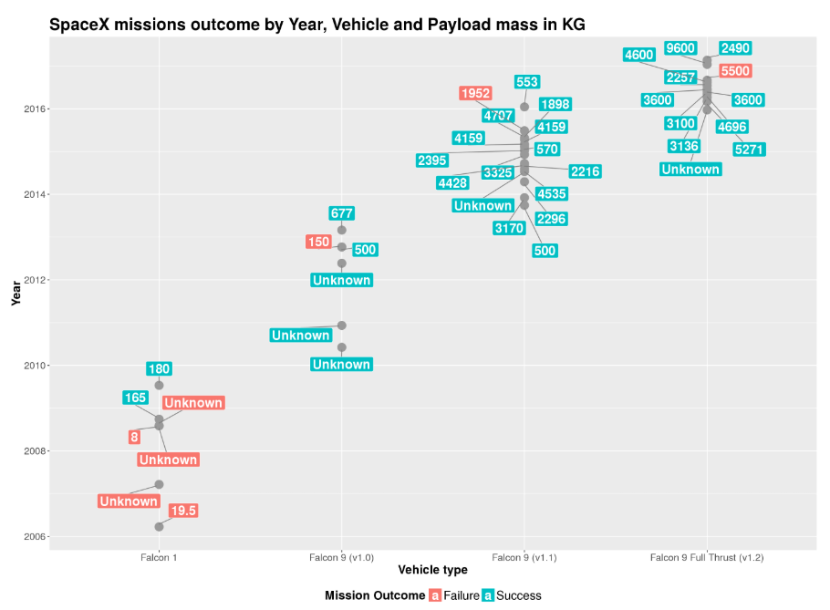
ggplot(dfS)+ geom_point(aes(VehicleType, LaunchDate), size = 5, color = 'grey60') +
  geom_label_repel(aes(VehicleType, LaunchDate, fill = ifelse(dfS$MissionOutcome == 'Failure', 'Failure', 'Success'),
        label = PayloadMasskg),fontface = 'bold', color = 'white', size = 6, box.padding = unit(0.35, "lines"),
        point.padding = unit(0.5, "lines"),segment.color = 'grey50') +
  ggtitle("SpaceX missions outcome by Year, Vehicle and Payload mass in KG")+ labs(x="Vehicle type",y="Year") +
  theme(legend.title = element_text(face = "bold", size = 16)) + theme(legend.text = element_text(size = 16)) +
  theme(legend.position = "bottom")+ labs(fill = "Mission Outcome") +
  theme(plot.title = element_text(size = 22, face = "bold")) +
  theme(axis.text=element_text(size=13), axis.title=element_text(size=16,face="bold"))

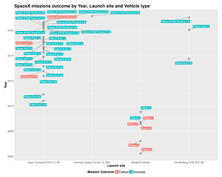
ggplot(dfS)+ geom_point(aes(LaunchSite, LaunchDate), size = 4, color = 'grey60') +
  geom_label_repel(aes(LaunchSite, LaunchDate, fill = ifelse(dfS$MissionOutcome == 'Failure', 'Failure', 'Success'),
       label = VehicleType), fontface = 'bold', color = 'white', size = 4, box.padding = unit(0.35, "lines"),
       point.padding = unit(0.5, "lines"),segment.color = 'grey50') +
  ggtitle("SpaceX missions outcome by Year, Launch site and Vehicle type")+ labs(x="Launch site",y="Year") +
  theme(legend.title = element_text(face = "bold", size = 16)) + theme(legend.text = element_text(size = 16)) +
  theme(legend.position = "bottom")+ labs(fill = "Mission Outcome") +
  theme(plot.title = element_text(size = 22, face = "bold")) +
  theme(axis.text=element_text(size=13), axis.title=element_text(size=16,face="bold"))

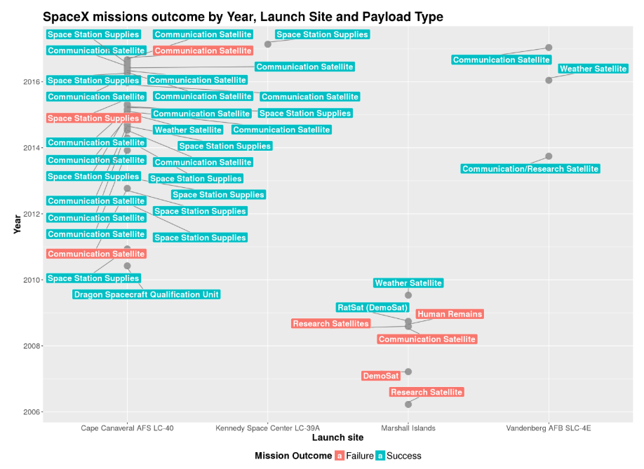
ggplot(dfS)+ geom_point(aes(LaunchSite, LaunchDate), size = 5, color = 'grey60') +
  geom_label_repel(aes(LaunchSite, LaunchDate, fill = ifelse(dfS$MissionOutcome == 'Failure', 'Failure', 'Success'),
      label = PayloadType), fontface = 'bold', color = 'white', size = 5, box.padding = unit(0.35, "lines"),
      point.padding = unit(0.5, "lines"),segment.color = 'grey50') +
  ggtitle("SpaceX missions outcome by Year, Launch Site and Payload Type")+ labs(x="Launch site",y="Year") +
  theme(legend.title = element_text(face = "bold", size = 16)) + theme(legend.text = element_text(size = 16)) +
  theme(legend.position = "bottom")+ labs(fill = "Mission Outcome") +
  theme(plot.title = element_text(size = 22, face = "bold")) +
  theme(axis.text=element_text(size=13), axis.title=element_text(size=16,face="bold"))

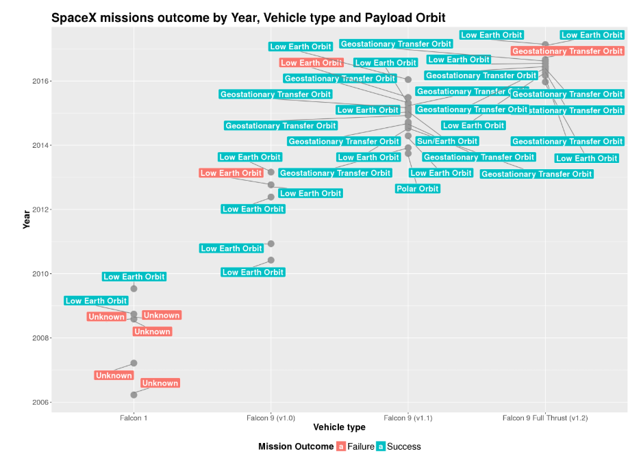
ggplot(dfS)+ geom_point(aes(VehicleType, LaunchDate), size = 5, color = 'grey60') +
  geom_label_repel(aes(VehicleType, LaunchDate, fill = ifelse(dfS$MissionOutcome == 'Failure', 'Failure', 'Success'),
      label = PayloadOrbit), fontface = 'bold', color = 'white', size = 5, box.padding = unit(0.35, "lines"),
      point.padding = unit(0.5, "lines"),segment.color = 'grey50') +
  ggtitle("SpaceX missions outcome by Year, Vehicle type and Payload Orbit")+  labs(x="Vehicle type",y="Year") +
  theme(legend.title = element_text(face = "bold", size = 16)) + theme(legend.text = element_text(size = 16)) +
  theme(legend.position = "bottom")+ labs(fill = "Mission Outcome") +
  theme(plot.title = element_text(size = 22, face = "bold")) +
  theme(axis.text=element_text(size=13), axis.title=element_text(size=16,face="bold"))

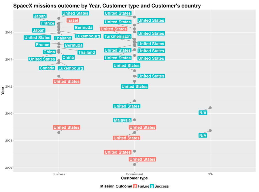
ggplot(dfS)+ geom_point(aes(CustomerType, LaunchDate), size = 5, color = 'grey60') +
  geom_label_repel(aes(CustomerType, LaunchDate, fill = ifelse(dfS$MissionOutcome == 'Failure', 'Failure', 'Success'),
      label = CustomerCountry), fontface = 'bold', color = 'white', size = 6, box.padding = unit(0.35, "lines"),
      point.padding = unit(0.5, "lines"),segment.color = 'grey50') +
  ggtitle("SpaceX missions outcome by Year, Customer type and Customer's country")+ labs(x="Customer type",y="Year") +
  theme(legend.title = element_text(face = "bold", size = 16)) + theme(legend.text = element_text(size = 16)) +
  theme(legend.position = "bottom")+ labs(fill = "Mission Outcome") +
  theme(plot.title = element_text(size = 22, face = "bold")) +
  theme(axis.text=element_text(size=13), axis.title=element_text(size=16,face="bold"))

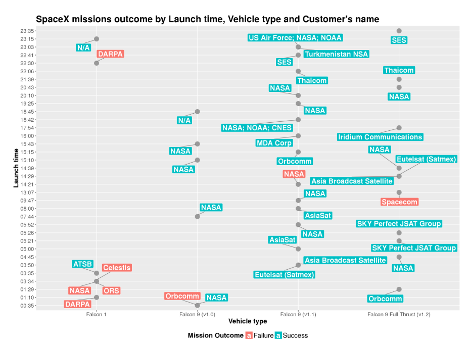
ggplot(dfS)+ geom_point(aes(VehicleType, LaunchTime), size = 5, color = 'grey60') +
  geom_label_repel(aes(VehicleType, LaunchTime, fill = ifelse(dfS$MissionOutcome == 'Failure', 'Failure', 'Success'),
      label = CustomerName), fontface = 'bold', color = 'white', size = 6, box.padding = unit(0.35, "lines"),
      point.padding = unit(0.5, "lines"),segment.color = 'grey50') +
  ggtitle("SpaceX missions outcome by Launch time, Vehicle type and Customer's name")+ labs(x="Vehicle type",y="Launch time") +
  theme(legend.title = element_text(face = "bold", size = 16)) + theme(legend.text = element_text(size = 16)) +
  theme(legend.position = "bottom")+ labs(fill = "Mission Outcome") +
  theme(plot.title = element_text(size = 22, face = "bold")) +
  theme(axis.text=element_text(size=13), axis.title=element_text(size=16,face="bold"))

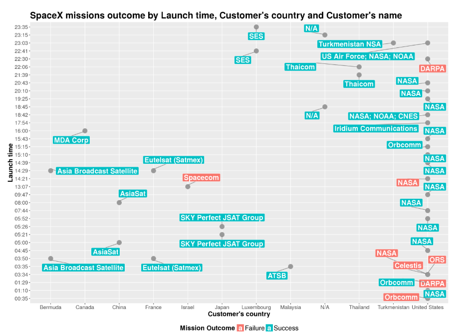
ggplot(dfS)+ geom_point(aes(CustomerCountry, LaunchTime), size = 5, color = 'grey60') +
  geom_label_repel(aes(CustomerCountry, LaunchTime, fill = ifelse(dfS$MissionOutcome == 'Failure', 'Failure', 'Success'),
      label = CustomerName), fontface = 'bold', color = 'white', size = 6, box.padding = unit(0.35, "lines"),
      point.padding = unit(0.5, "lines"),segment.color = 'grey50') +
  ggtitle("SpaceX missions outcome by Launch time, Customer's country and Customer's name")+
  labs(x="Customer's country",y="Launch time") +
  theme(legend.title = element_text(face = "bold", size = 16)) + theme(legend.text = element_text(size = 16)) +
  theme(legend.position = "bottom")+ labs(fill = "Mission Outcome") +
  theme(plot.title = element_text(size = 22, face = "bold")) +
  theme(axis.text=element_text(size=13), axis.title=element_text(size=16,face="bold"))

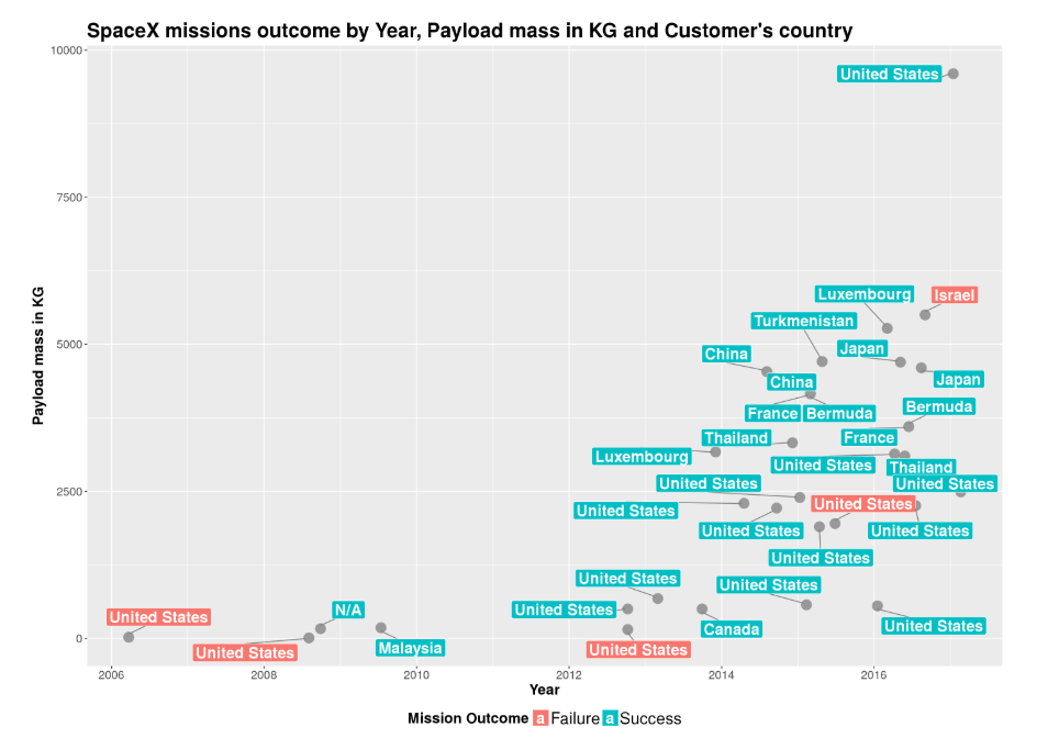
dfS$PayloadMasskg = as.integer(dfS$PayloadMasskg)

ggplot(dfS)+ geom_point(aes(LaunchDate, PayloadMasskg), size = 5, color = 'grey60') +
  geom_label_repel(aes(LaunchDate, PayloadMasskg, fill = ifelse(dfS$MissionOutcome == 'Failure', 'Failure', 'Success'),
      label = CustomerCountry), fontface = 'bold', color = 'white', size = 6, box.padding = unit(0.35, "lines"),
      point.padding = unit(0.5, "lines"),segment.color = 'grey50') +
  ggtitle("SpaceX missions outcome by Year, Payload mass in KG and Customer's country")+ labs(x="Year",y="Payload mass in KG") +
  theme(legend.title = element_text(face = "bold", size = 16)) + theme(legend.text = element_text(size = 18)) +
  theme(legend.position = "bottom")+ labs(fill = "Mission Outcome") +
  theme(plot.title = element_text(size = 22, face = "bold")) +
  theme(axis.text=element_text(size=13), axis.title=element_text(size=16,face="bold"))