吴裕雄--天生自然 R语言数据可视化绘图（1）

par(ask=TRUE)
opar <- par(no.readonly=TRUE) # make a copy of current settings

attach(mtcars) # be sure to execute this line

plot(wt, mpg)
abline(lm(mpg~wt))
title("Regression of MPG on Weight")

# Input data for drug example
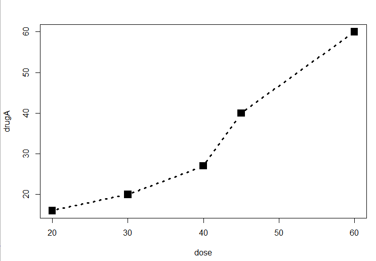
dose  <- c(20, 30, 40, 45, 60)
drugA <- c(16, 20, 27, 40, 60)
drugB <- c(15, 18, 25, 31, 40)

plot(dose, drugA, type="b")

opar <- par(no.readonly=TRUE) # make a copy of current settings
par(lty=2, pch=17)            # change line type and symbol
plot(dose, drugA, type="b")   # generate a plot
par(opar)                     # restore the original settings 

plot(dose, drugA, type="b", lty=3, lwd=3, pch=15, cex=2)

# choosing colors
library(RColorBrewer)
n <- 7
mycolors <- brewer.pal(n, "Set1")
barplot(rep(1,n), col=mycolors)

n <- 10
mycolors <- rainbow(n)
pie(rep(1, n), labels=mycolors, col=mycolors)
mygrays <- gray(0:n/n)
pie(rep(1, n), labels=mygrays, col=mygrays)

dose <- c(20, 30, 40, 45, 60)
drugA <- c(16, 20, 27, 40, 60)
drugB <- c(15, 18, 25, 31, 40)
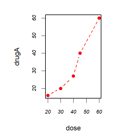
opar <- par(no.readonly=TRUE)
par(pin=c(2, 3))
par(lwd=2, cex=1.5)
par(cex.axis=.75, font.axis=3)
plot(dose, drugA, type="b", pch=19, lty=2, col="red")
plot(dose, drugB, type="b", pch=23, lty=6, col="blue", bg="green")
par(opar)

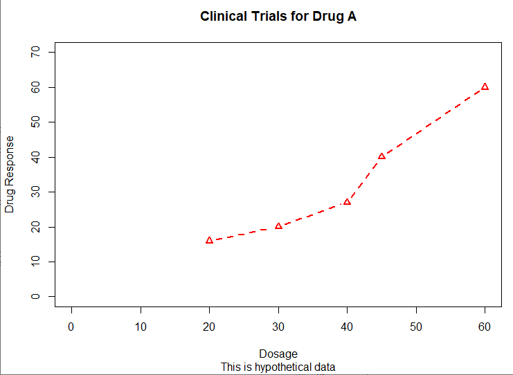
# Adding text, lines, and symbols
plot(dose, drugA, type="b",
     col="red", lty=2, pch=2, lwd=2,
     main="Clinical Trials for Drug A",
     sub="This is hypothetical data",
     xlab="Dosage", ylab="Drug Response",
     xlim=c(0, 60), ylim=c(0, 70))

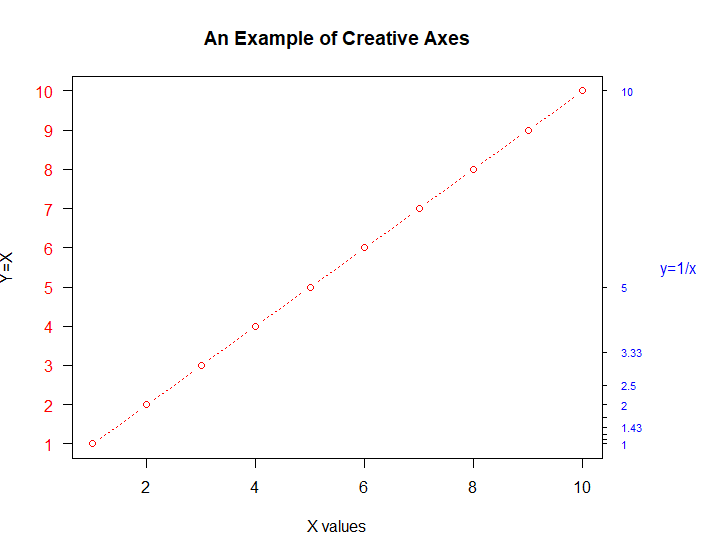
x <- c(1:10)
y <- x
z <- 10/x
opar <- par(no.readonly=TRUE)
par(mar=c(5, 4, 4, 8) + 0.1)
plot(x, y, type="b",
     pch=21, col="red",
     yaxt="n", lty=3, ann=FALSE)
lines(x, z, type="b", pch=22, col="blue", lty=2)
axis(2, at=x, labels=x, col.axis="red", las=2)
axis(4, at=z, labels=round(z, digits=2),
     col.axis="blue", las=2, cex.axis=0.7, tck=-.01)
mtext("y=1/x", side=4, line=3, cex.lab=1, las=2, col="blue")
title("An Example of Creative Axes",
      xlab="X values",
      ylab="Y=X")
par(opar)

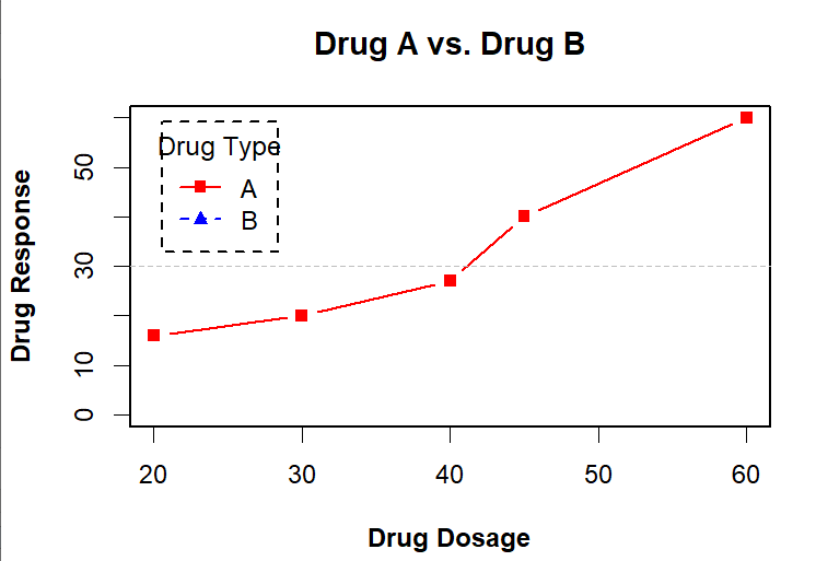
dose <- c(20, 30, 40, 45, 60)
drugA <- c(16, 20, 27, 40, 60)
drugB <- c(15, 18, 25, 31, 40)
opar <- par(no.readonly=TRUE)
par(lwd=2, cex=1.5, font.lab=2)
plot(dose, drugA, type="b",
     pch=15, lty=1, col="red", ylim=c(0, 60),
     main="Drug A vs. Drug B",
     xlab="Drug Dosage", ylab="Drug Response")
lines(dose, drugB, type="b",
      pch=17, lty=2, col="blue")
abline(h=c(30), lwd=1.5, lty=2, col="gray")
library(Hmisc)
minor.tick(nx=3, ny=3, tick.ratio=0.5)
legend("topleft", inset=.05, title="Drug Type", c("A","B"),
       lty=c(1, 2), pch=c(15, 17), col=c("red", "blue"))
par(opar)

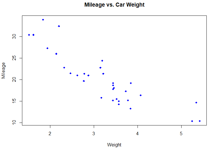
attach(mtcars)
plot(wt, mpg,
     main="Mileage vs. Car Weight",
     xlab="Weight", ylab="Mileage",
     pch=18, col="blue")
text(wt, mpg,
     row.names(mtcars),
     cex=0.6, pos=4, col="red")
detach(mtcars)

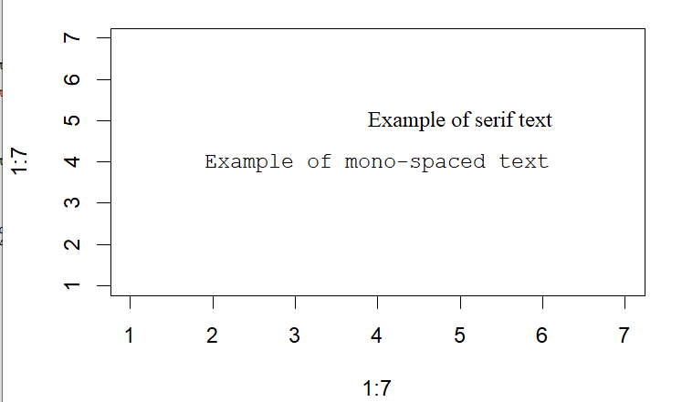
# View font families
opar <- par(no.readonly=TRUE)
par(cex=1.5)
plot(1:7,1:7,type="n")
text(3,3,"Example of default text")
text(4,4,family="mono","Example of mono-spaced text")
text(5,5,family="serif","Example of serif text")
par(opar)

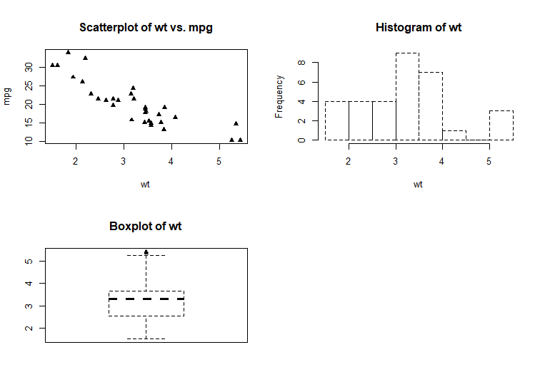
# Combining graphs
attach(mtcars)
opar <- par(no.readonly=TRUE)
par(mfrow=c(2,2))
plot(wt,mpg, main="Scatterplot of wt vs. mpg")
plot(wt,disp, main="Scatterplot of wt vs. disp")
hist(wt, main="Histogram of wt")
boxplot(wt, main="Boxplot of wt")
par(opar)
detach(mtcars)

attach(mtcars)
opar <- par(no.readonly=TRUE)
par(mfrow=c(3,1))
hist(wt)
hist(mpg)
hist(disp)
par(opar)
detach(mtcars)

attach(mtcars)
layout(matrix(c(1,1,2,3), 2, 2, byrow = TRUE))
hist(wt)
hist(mpg)
hist(disp)
detach(mtcars)

attach(mtcars)
layout(matrix(c(1, 1, 2, 3), 2, 2, byrow = TRUE),
       widths=c(3, 1), heights=c(1, 2))
hist(wt)
hist(mpg)
hist(disp)
detach(mtcars)

# Listing 3.4 - Fine placement of figures in a graph
opar <- par(no.readonly=TRUE)
par(fig=c(0, 0.8, 0, 0.8))
plot(mtcars$mpg, mtcars$wt,
     xlab="Miles Per Gallon",
     ylab="Car Weight")
par(fig=c(0, 0.8, 0.55, 1), new=TRUE)
boxplot(mtcars$mpg, horizontal=TRUE, axes=FALSE)
par(fig=c(0.65, 1, 0, 0.8), new=TRUE)
boxplot(mtcars$wt, axes=FALSE)
mtext("Enhanced Scatterplot", side=3, outer=TRUE, line=-3)
par(opar)